UAV Systems Engineering · Module 2
M2-T5: GNSS signal blockage
You can predict where GNSS will fail from a skyline: the satellites you cannot see are the ones that do not count.
GNSS-denied navigation is rarely “no signal”: it is a gradual loss of satellites and geometry as the vehicle enters a canyon, a tunnel, a warehouse or a forest. This lesson shows how to predict and detect that loss early enough to act.
Learning objectives
After this lesson, you should be able to:
- Explain how obstruction reduces satellite count and geometry.
- Compute availability and HDOP from a skyline profile.
- Use satellite count, DOP and C/N0 as early-warning indicators.
- Set thresholds that trigger the GNSS-degraded modes of module 8.
Conceptual explanation
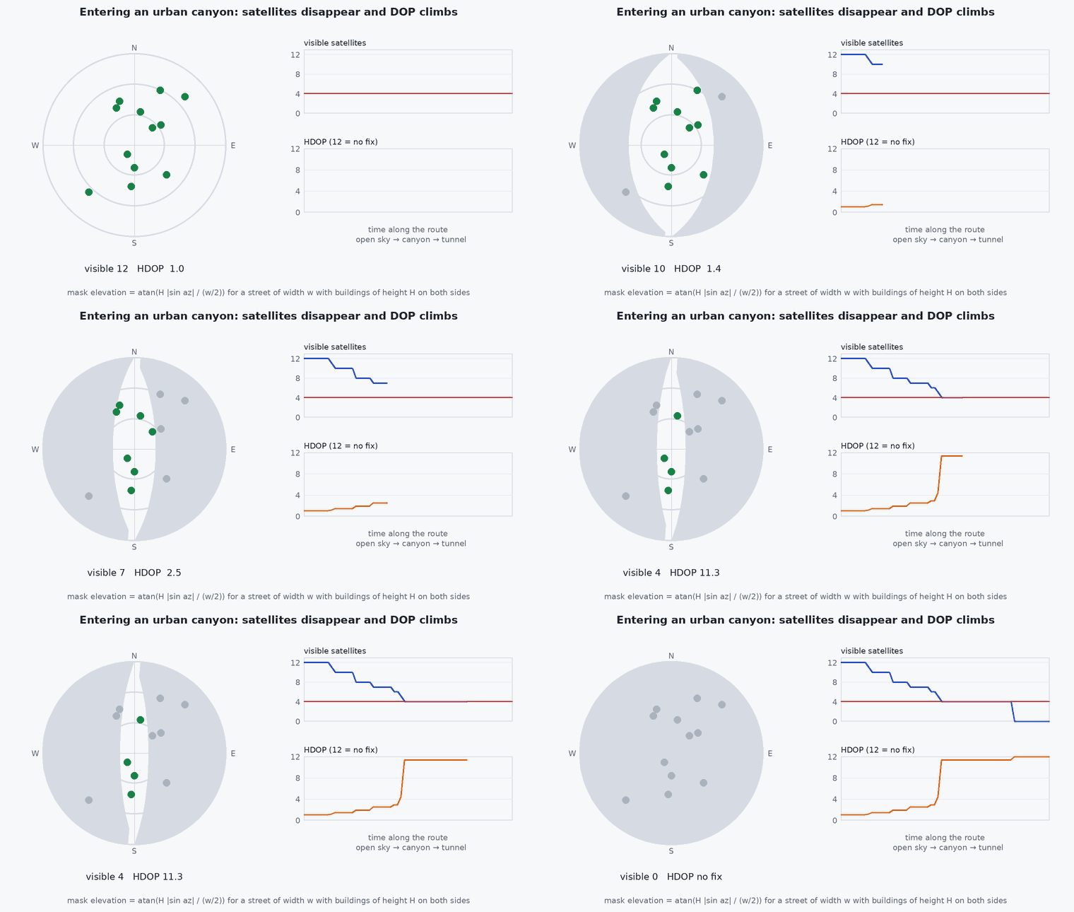
Buildings, terrain, foliage and roofs block or attenuate signals. A satellite is usable only if the line of sight is clear above the skyline (the elevation of the obstruction in each azimuth) and the receiver’s elevation mask. Indoors, almost nothing is visible; under canopy, signals are attenuated and noisy; in a street canyon, the visible sky is a narrow slot along the street direction, which gives poor geometry in the cross-street direction.
Engineering intuition
In a canyon aligned north–south, satellites to the east and west are hidden and those along the street are visible, so the along-street position is well determined and the cross-street position is poorly determined. DOP captures this directionally: HDOP is large even if the satellite count is acceptable. Count alone is a poor indicator; geometry matters. Also remember the transition: the receiver loses satellites over seconds while the vehicle is moving, so the monitor should react to trends (count falling, DOP rising) and give the estimator time to switch.
Mathematical formulation
Visibility of a satellite at azimuth A and elevation : (mask, skyline(A)). With line-of-sight unit vectors (east, north, up) of the visible satellites, the horizontal dilution of precision is obtained from the 3-D geometry matrix with a clock column:
Availability is the fraction of time (or positions) with at least four satellites and HDOP below a threshold. Required HDOP follows from the accuracy requirement: ≈ HDOP × , so a 2 m position requirement with needs HDOP below about 1.3.
- skyline(A)
- elevation angle of the obstruction at azimuth A.
- effective user range error (m).
Architecture and data flow
The receiver outputs satellite count, DOP and per-satellite C/N0 and elevation; the monitor trends them and sets a trust flag with hysteresis (lesson M8-T11). Maps of expected availability can be computed in advance from a 3-D building model and an almanac for mission planning: plan the route so that predicted GNSS-poor segments coincide with segments where odometry is strong.
Real-world UAV applications
- Mission planning through urban canyons.
- Choosing sensors for tunnels, warehouses and forests.
- Setting the GNSS-loss thresholds of the failsafe logic.
- Explaining why GNSS “worked in the field test” but not near the real site.
Implementation example
This runs as shown: HDOP and availability for a street canyon (obstruction on both sides) at several street widths and building heights, using a synthetic satellite sky.
import numpy as np
rng = np.random.default_rng(5)

def sky(n):
    az = rng.uniform(0, 2 * np.pi, n); el = np.arcsin(rng.uniform(0, 1, n)); return az, el

def canyon_skyline(az, street_az_deg, half_width_m, building_h_m):
    """Elevation of the buildings along azimuth az for a receiver in the middle of a straight street."""
    rel = az - np.radians(street_az_deg)
    cross = np.abs(np.sin(rel))                                     # 0 along the street, 1 across it
    dist = np.where(cross < 1e-3, 1e9, half_width_m / np.maximum(cross, 1e-3))      # distance to the facade along this azimuth
    return np.arctan2(building_h_m, dist)

def hdop(az, el):
    u = np.stack([np.cos(el) * np.sin(az), np.cos(el) * np.cos(az), np.sin(el)], axis=1)
    H = np.hstack([-u, np.ones((len(u), 1))])
    if len(u) < 4 or np.linalg.matrix_rank(H) < 4: return np.inf
    Q = np.linalg.inv(H.T @ H); return np.sqrt(Q[0, 0] + Q[1, 1])

def availability(half_width, height, trials=400, nsat=40, mask=10, thresh=3.0):
    ok, hs = 0, []
    for _ in range(trials):
        az, el = sky(nsat); vis = el > np.maximum(np.radians(mask), canyon_skyline(az, 0.0, half_width, height))
        h = hdop(az[vis], el[vis]); hs.append(h); ok += np.isfinite(h) and h < thresh
    return ok / trials, np.median([h for h in hs if np.isfinite(h)] or [np.inf])

open_sky = availability(1e6, 0.0); wide = availability(25.0, 20.0); narrow = availability(8.0, 40.0)
print("open sky (avail, median HDOP):", np.round(open_sky, 2), "| wide street:", np.round(wide, 2), "| narrow canyon:", np.round(narrow, 2))
assert open_sky[0] > 0.98 and narrow[0] < wide[0] <= open_sky[0] and narrow[1] > wide[1] > 0.9 * open_sky[1]Common engineering mistakes
Using satellite count alone
Geometry matters: a canyon can show ten satellites and a bad HDOP.
Setting thresholds from open-sky tests
Test in the real environment, including the transitions.
Reacting to a single epoch
Use trends and hysteresis to avoid chatter.
Forgetting reflections
In a canyon, non-line-of-sight signals can be tracked and be wrong by tens of metres even with good count and DOP.
No plan for the exit
Re-acquisition after a tunnel needs a bounded, smooth correction (lesson M8-T11).
Failure modes
| Failure mode | How it shows up | Likely cause |
|---|---|---|
| Non-line-of-sight positioning | Smooth but wrong position near tall buildings | Reflected signals treated as direct |
| Slow loss | Count decays over seconds | Entering a canyon or tunnel |
| Sudden jump on exit | Position steps when GNSS returns | Re-acquisition after drift |
| False GNSS-denied alarm | Mode changes in good conditions | Thresholds from the wrong environment |
Debugging approach
- Plot satellites, HDOP and C/N0 with the path on a map.
- Compare the predicted skyline mask with observed satellite visibility.
- Record transitions at several speeds.
- Check consistency against odometry to spot non-line-of-sight errors (lesson M2-T6).
Practical exercises
- Compute the skyline elevation for a 30 m building at 10 m from the receiver.
- Find the street half-width at which availability falls below 90% for 30 m buildings.
- Add a mask of and compare.
- Propose thresholds on count, HDOP and C/N0 for a monitor and justify them.
Interview questions
Write an answer in your own words, then reveal the model answer. Nothing is sent anywhere.
Question 1
Why is satellite count a poor indicator of GNSS quality?
Model answer
Geometry matters: satellites clustered along one direction give a large DOP even with many in view, and reflected signals can be counted while being wrong.
Question 2
How can you predict GNSS availability along a route?
Model answer
From a 3-D model of obstructions and the satellite almanac: compute visible satellites and DOP along the path.
Question 3
What should the monitor look at?
Model answer
Satellite count, DOP and per-satellite C/N0 with their trends, plus cross-checks against odometry, with hysteresis on mode changes.
References and further reading
Primary papers, official documentation and standards. Each claim above that is specific to a tool or version points here.
- . . Groves, Principles of GNSS, Inertial, and Multisensor Integrated Navigation Systems, 2nd ed., Artech House, 2013, chapter 9 (urban positioning).
- ESA Navipedia: DOP and GNSS performance
- PX4: EKF2 GNSS quality checks