UAV Systems Engineering · Module 6
M6-T5: PX4 state estimation and EKF2
EKF2 decides what the vehicle believes. Know its sources, its gates and its health signals before blaming the controller.
Almost every “the drone flew badly” report is an estimation problem in disguise. PX4 runs an extended Kalman filter (EKF2) that fuses the IMU with several optional sources. Knowing which sources are active, how each is gated, and how to read its innovations is the single most useful debugging skill for this stack.
Learning objectives
After this lesson, you should be able to:
- List the sources EKF2 can fuse and the parameters that enable them in your release.
- Interpret innovation test ratios, status flags and resets in the log.
- Explain how delays, noise and gating parameters affect behaviour.
- Diagnose a bad estimate to its source: vibration, magnetometer, GNSS or external vision.
Conceptual explanation
Implementation-specific EKF2 parameter names and message names change between PX4 releases (for example the older EKF2_AID_MASK was replaced by per-source control parameters such as EKF2_GPS_CTRL and EKF2_EV_CTRL in newer versions). Read the “Using the ECL EKF” page of the documentation for the version you fly. Parameter names below are examples to look up, not a fixed contract.
EKF2 is an error-state extended Kalman filter derived from the ECL library: the IMU integrates the nominal state at high rate, and a covariance-propagating filter estimates the error state, correcting it with aiding measurements: GNSS position and velocity, barometric height, magnetometer heading or yaw, rangefinder, optical flow, airspeed (fixed wing) and external vision (position, velocity, yaw). It also estimates IMU biases and, optionally, wind and magnetic field states.
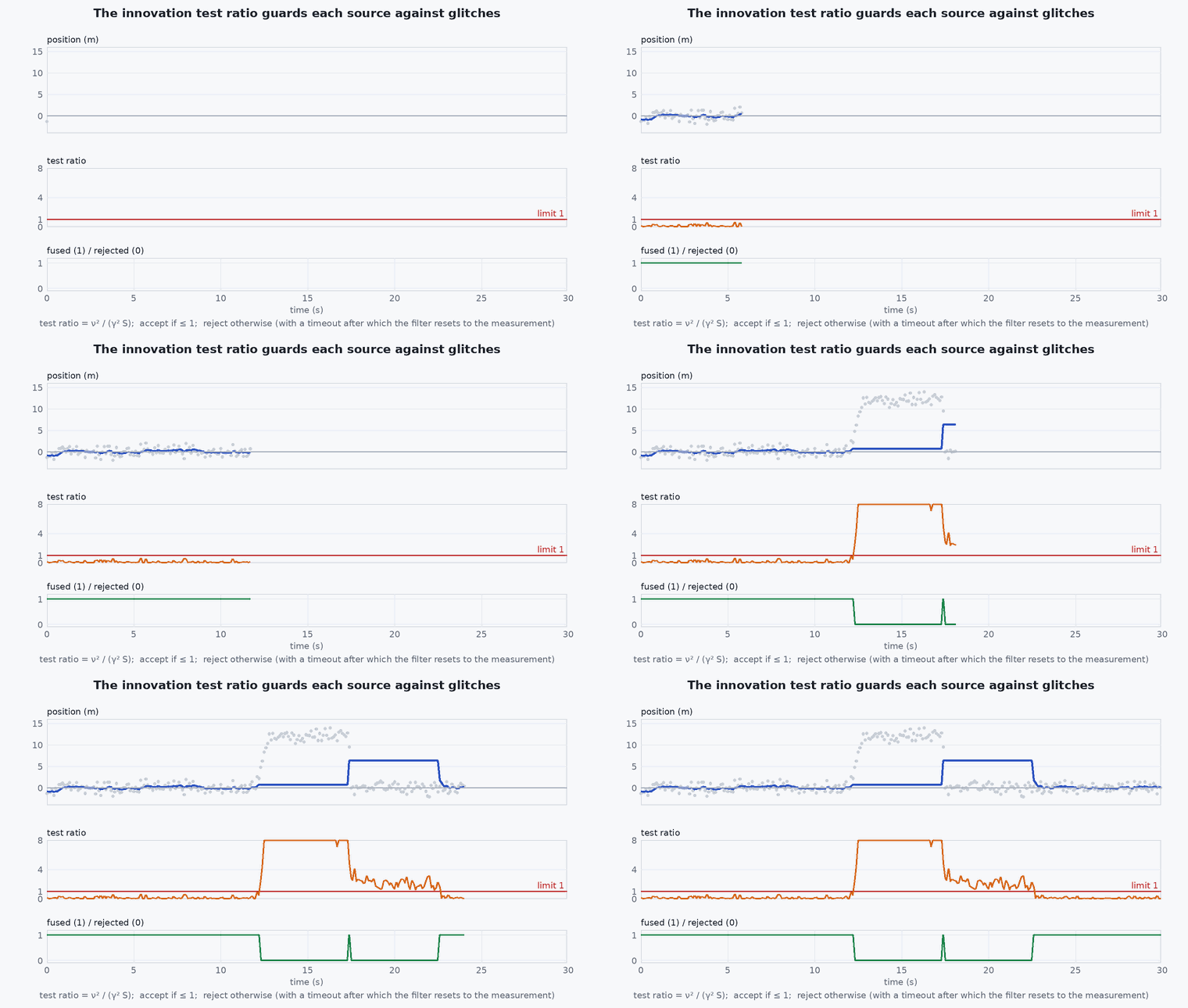
Each aiding source goes through the same process: the measurement is compared to the prediction, the innovation is normalised by its predicted covariance, and if the squared normalised value exceeds a gate (a number of standard deviations, set by a parameter) the measurement is rejected. Persistent rejection leads to a timeout, a reset of the estimate toward the measurement, or a failsafe. Several parameters control each source: its noise, its gate, its delay relative to the IMU, and whether it is used at all.
Engineering intuition
The filter is a weighted average of a model prediction and measurements, with the weights set by the covariances. Tell it a sensor is more accurate than it is (noise parameter too small) and it will believe it too much and be dragged around by errors; tell it the sensor is noisy and it will trust the IMU and drift. Gates are the safety net: a measurement that is wildly inconsistent is thrown away instead of accepted.
When the estimate is wrong, find the source of the inconsistency. High vibration clips the accelerometer and corrupts the prediction (look at the vibration metrics and the innovation test ratios of velocity and height). A magnetic disturbance appears in heading innovation. A bad GNSS fix appears as position and velocity innovations that grow. External vision with a wrong frame or time offset appears as a position innovation that correlates with vehicle motion.
Mathematical formulation
For a measurement with prediction and innovation covariance , the innovation and the test ratio are
EKF2 reports these ratios as estimator_status test ratios (for example velocity, horizontal position, vertical position, magnetometer, height above ground); values below 1 mean the fusion is accepted, values persistently near or above 1 mean the filter and the source disagree. A measurement delay of seconds relative to the IMU is handled by a buffer: the measurement is compared with the state at time , so a wrong delay parameter turns motion into apparent innovation:
At 5 m/s a 100 ms delay error already gives 0.5 m of spurious innovation, comparable to a good GNSS accuracy; that is why delay parameters (for example the external-vision delay) must be measured, not guessed.
- ,
- innovation and its covariance.
- gate in standard deviations (a parameter per source).
- error in the assumed measurement delay (s).
Architecture and data flow
IMU (integrated through the IMU prediction) + aiding sources → ekf2 → vehicle_local_position, vehicle_global_position, vehicle_attitude, vehicle_odometry; health in estimator_status (and in newer releases the estimator_status_flags, estimator_innovations and related topics), failsafe-relevant flags in vehicle_status. The controllers and navigator consume the outputs; the commander reads the validity flags for mode checks and failsafes.
Real-world UAV applications
- Choosing which sources a vehicle should fuse in a GNSS-denied test.
- Diagnosing drift and glitches in position hold.
- Setting up external vision with the right delay and noise.
- Deciding when to declare the estimate unusable and trigger a failsafe.
Implementation example
This runs as shown. A reduced model of the mechanism: a 10 Hz position measurement of where the vehicle was 100 ms ago is compared with the filter’s own position estimate at the time the filter assumes the measurement was taken. The normalised innovation is at the noise level only when the assumed delay is right, which also gives a practical way to measure the delay: scan the assumed delay and take the minimum. It is a model of the mechanism, not EKF2 code.
import numpy as np
rng = np.random.default_rng(1)
dt, n = 0.01, 6000
t = np.arange(n) * dt
p_true = 10.0 * np.sin(0.8 * t)                                  # moving vehicle, peak speed 8 m/s
true_delay, sigma, sigma_est = 0.10, 0.20, 0.10
p_est = p_true + sigma_est * rng.standard_normal(n)              # the filter's own (undelayed) position estimate, accurate to about 0.1 m
k_meas = np.arange(300, n, 10)                                   # a 10 Hz position measurement of where the vehicle was true_delay ago
z = p_true[k_meas - int(round(true_delay / dt))] + sigma * rng.standard_normal(k_meas.size)

def mean_nis(assumed_delay):
    ka = k_meas - int(round(assumed_delay / dt))                 # compare with the estimate at the time we BELIEVE the measurement was taken
    nu = z - p_est[ka]; return float(np.mean(nu ** 2 / (sigma ** 2 + sigma_est ** 2)))
delays = np.arange(0.0, 0.31, 0.02)
nis = np.array([mean_nis(d) for d in delays])
best = delays[np.argmin(nis)]
print(f"mean NIS: delay right {mean_nis(0.10):.2f}, delay ignored {mean_nis(0.0):.2f}; delay scan minimum at {best:.2f} s")
assert mean_nis(0.0) > 2.0 * mean_nis(0.10) and abs(best - 0.10) < 0.021 and mean_nis(0.10) < 1.5Common engineering mistakes
Leaving external-vision delay at the default
Measure it; a wrong delay looks like a noisy source.
Loosening gates to hide a problem
The filter then accepts bad data; fix the source.
Ignoring vibration
Accelerometer clipping corrupts everything that follows; check vibration metrics first.
Enabling several sources without a plan
Conflicting sources fight each other; decide the primary source per axis.
Not checking resets
Position and heading resets move the setpoint frame under the controller.
Failure modes
| Failure mode | How it shows up | Likely cause |
|---|---|---|
| Position drift in hold | Slow wander | Weak aiding source, wrong noise parameters, bias not observable |
| Sudden jumps | Position or yaw reset | Source change, gate timeout, GNSS glitch, EV frame mismatch |
| Height oscillation | Vertical bobbing | Barometer pressure error from airflow or vibration; rangefinder conflicts |
| Failsafe on estimator error | Switches to land or hold | Test ratios exceeded for the timeout period |
Debugging approach
- Plot the innovation test ratios and status flags with the position error.
- Check vibration metrics and accelerometer clipping first.
- Compare each source against the estimate to find the offender.
- Log and review resets (counter changes) around the event time.
Practical exercises
- In a log, find the time EKF2 started fusing GNSS after takeoff and the flags that changed.
- Disable GNSS fusion in SITL (parameter for your version) and watch the estimate degrade.
- Compute the position error from a 60 ms delay error at 10 m/s.
- Plot the velocity innovation test ratio during an aggressive manoeuvre.
Interview questions
Write an answer in your own words, then reveal the model answer. Nothing is sent anywhere.
Question 1
What is an innovation test ratio?
Model answer
The squared normalised difference between a measurement and its prediction, divided by the gate; below 1 means the measurement is accepted, persistently high means the source and the filter disagree.
Question 2
Why does a wrong sensor delay show up as a noisy sensor?
Model answer
The filter compares the measurement with the state at the wrong time; the discrepancy scales with speed, so it looks like noise that grows with motion.
Question 3
How do you diagnose an EKF2 position glitch?
Model answer
Check resets and status flags at the time, plot innovation ratios of each source, check vibration and magnetometer health, and compare each aiding source with the estimate.
References and further reading
Primary papers, official documentation and standards. Each claim above that is specific to a tool or version points here.