Design & Selection · Module 02
LiDAR: 2D, 3D, spinning, solid-state, flash, FMCW
LiDAR gives direct metric geometry independent of ambient light. The architecture decides coverage, density, motion distortion and how it fails in rain, on glass and next to other LiDARs.
Assumptions: ROS 2 Jazzy. Class-level engineering guidance and tested arithmetic; the numbers in the worked examples are illustrations, not a product. Manufacturer specifications are included only where they were read from the manufacturer’s own datasheet or specification page, each with its source and date; every other field says “Not yet verified in this build”.
1. Engineering problem
A LiDAR measures distance by light. The question is rarely “which is best” but which architecture survives your failure case: glass doors, rain, dust, fast rotation, long range, a 0.9 m doorway or a person walking beside a vehicle. This guide separates the architectures, explains the physics behind each limit, connects the sensor to ROS 2 correctly (including what the standard messages do not contain), and gives a workflow and a lab to validate a unit instead of trusting a headline figure. New to LiDAR? Start with how each type works, with videos to watch.
2. When is this needed?
- Choosing a LiDAR type for an indoor robot, an outdoor vehicle, a drone or a humanoid.
- Explaining why a sensor behaves differently in the field from its bench result.
- Integrating a new LiDAR with ROS 2 Jazzy and validating it before deployment.
- Debugging distorted clouds, missing points, drift or dropped messages.
3. Selection and design decisions
Architectures at a glance
| Architecture | How the beam is steered | Moving parts | Field of view (tendency) | Range (tendency) | Typical strengths | Typical limits |
|---|---|---|---|---|---|---|
| 2D scanning | One emitter/receiver scanned through a plane by a rotating element | Yes: rotating mirror or head | Planar, often 270° or 360° | Metres to tens of metres (model dependent) | Cheap, light compute, mature ROS and Nav2 support | Single plane only; blind to anything above or below it |
| Mechanical spinning 3D | Many emitter/receiver channels on a rotating assembly (or a rotating mirror) | Yes: the whole sensor head or a large mirror rotates | 360° horizontal × tens of degrees vertical | Tens to hundreds of metres | Wide coverage, dense near-field geometry | Cost, wear and shock sensitivity; sparse at range between channels |
| MEMS-mirror scanning | A micro-mirror oscillates to scan the beam | Small moving parts (the mirror), no large rotation | Limited per unit (tens of degrees) | Tens to hundreds of metres | Compact, automotive-friendly | Narrow field of view per unit; mirror size limits optical aperture |
| Optical phased array (OPA) | Phase control across emitter elements steers the beam electronically | None in the scanning element | Limited by grating lobes and steering range | Typically shorter (research and early products) | No mechanical scanning | Optical loss, side lobes and limited power per element; less mature |
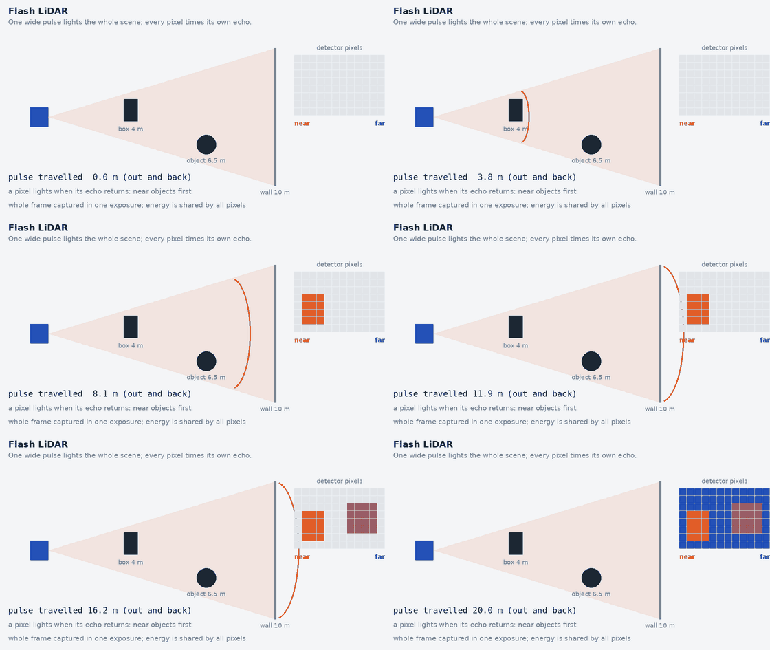
| Flash | The whole scene is illuminated at once; a detector array records all pixels simultaneously | None | Fixed by optics (often narrow to moderate) | Typically shorter than scanning types | Whole frame captured at one instant (no scan distortion); simple mechanics | Eye-safe pulse energy is spread over all pixels, so signal per pixel is low; ambient light sensitive |
| Hybrid / non-repetitive | A small number of moving elements produce a scan pattern that does not repeat each frame | Yes (small), by design | Wide for some models, narrow for others | Model dependent | Dense coverage builds up over integration time | Single-frame coverage is sparse; algorithms must accept the pattern |
| FMCW (4D) | Frequency-modulated continuous wave with coherent detection; beam steered by any of the above | Depends on the steering method | Model dependent | Model dependent | Range and radial velocity per point in one measurement | Cost, maturity and vendor-specific data formats; not immune to weather or interference |
“Solid-state” is a label, not a single technology. Flash and optical-phased-array designs have no moving scanning element; MEMS designs move a micro-mirror; hybrid designs keep a small rotating or oscillating element. Do not assume a product sold as solid-state has no moving parts: read how the beam is steered in its documentation.
Working principle at a glance, with videos to watch
About the videos. Each link was confirmed to be a real YouTube video (title and channel as YouTube reports them, checked 2026-11-05). I could not watch them or read their captions, so I only say what the title and channel support; check that a video suits you before relying on it. Several are made by LiDAR manufacturers, who explain their own approach favourably. The links open YouTube; nothing is embedded, so no YouTube content loads on this page.
All pulsed (time-of-flight) LiDAR
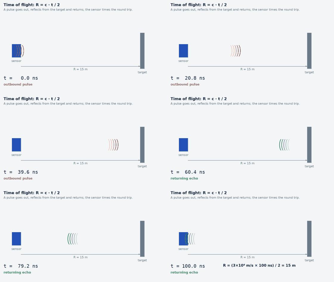
- What Is LiDAR? Time-of-Flight, 2D vs 3D Explained (with Real Outdoor Tests) · SICK Sensor Intelligence · 3:45 (by a 2D scanner manufacturer)
- What Is LiDAR and how does LiDAR work? · Phoenix LiDAR Systems · 6:04 (general introduction)
2D scanning LiDAR
LaserScan.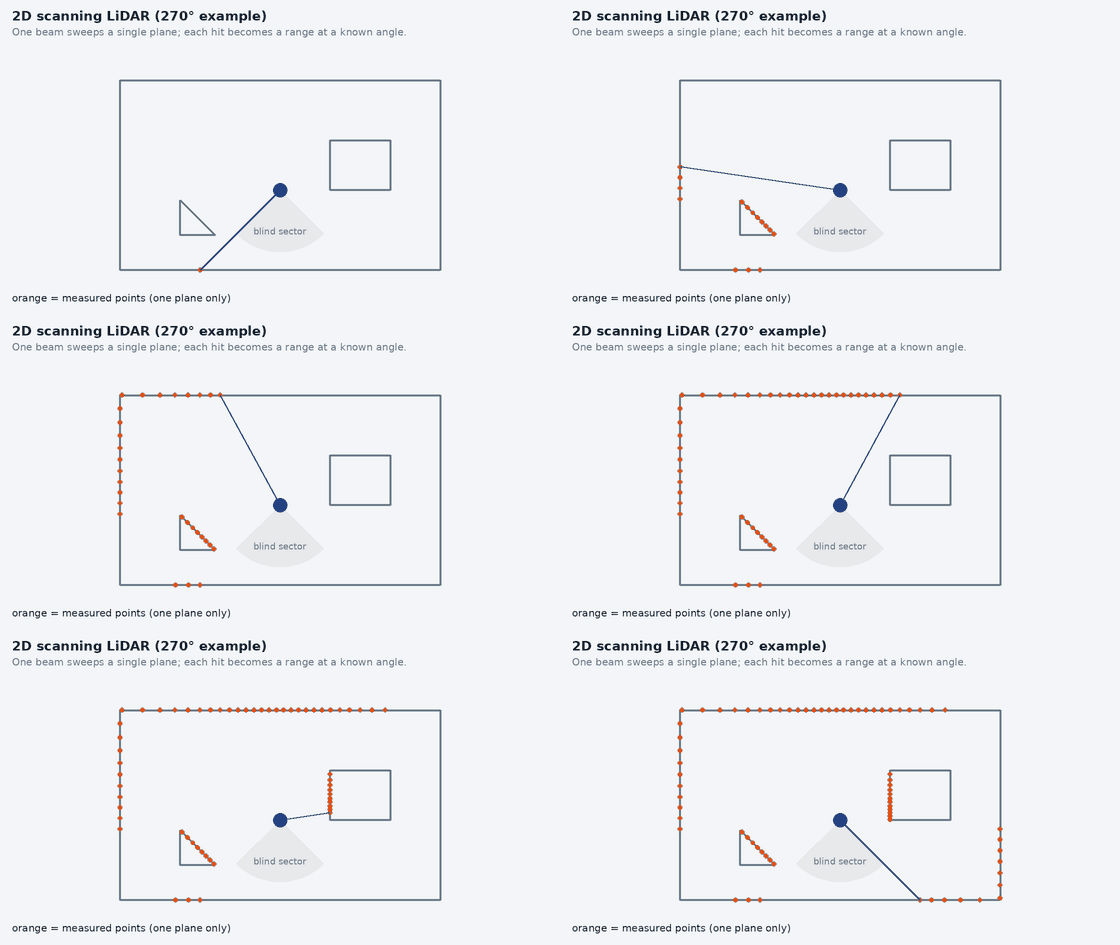
- What Is LiDAR? Time-of-Flight, 2D vs 3D Explained (with Real Outdoor Tests) · SICK Sensor Intelligence · 3:45 (by a 2D scanner manufacturer)
The first video also compares 2D and 3D, per its title.
Mechanical spinning 3D LiDAR
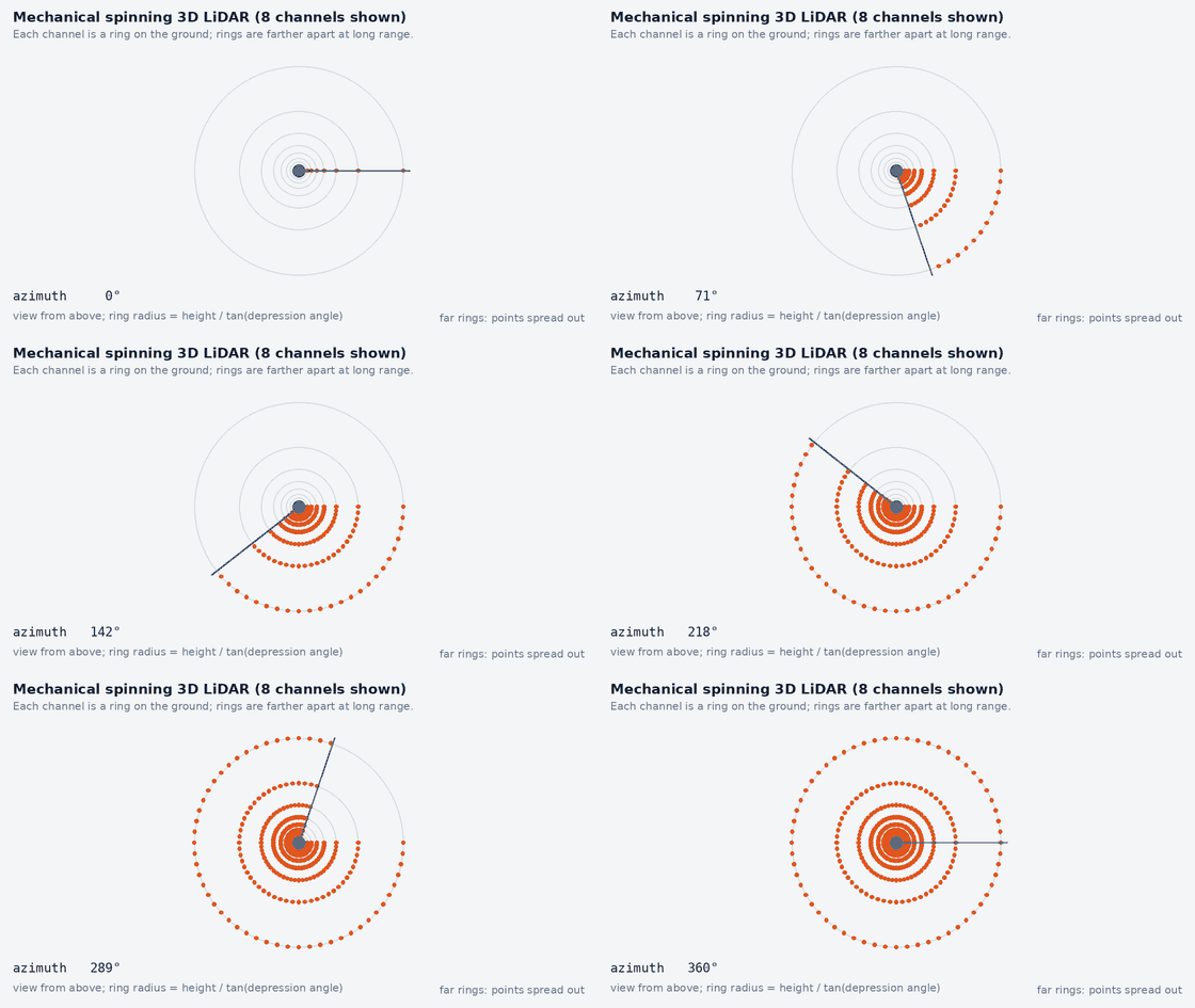
- How Ouster Digital Lidar works · Ouster · 0:53 (by the manufacturer: a short promotional overview)
- Lidar Technologies 101 · Hesai Technology · 7:06 (by a manufacturer: a technology overview that is not neutral about its own products)
MEMS-mirror LiDAR
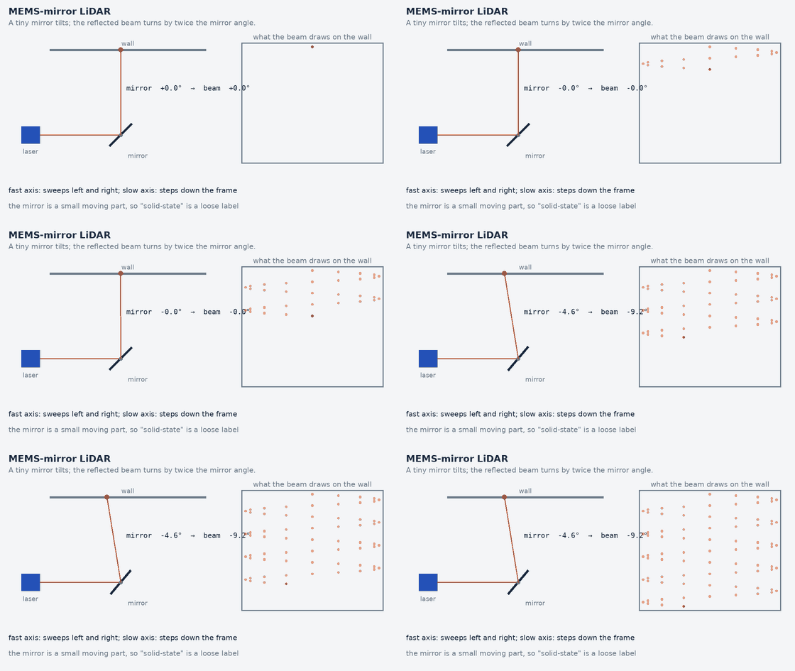
- The MEMS Solid-State LiDAR’s Principle & Features, RS-LiDAR-M1 Preview · RoboSense · 1:48 (by the manufacturer)
- MEMS Mirror Technologies of Fraunhofer IPMS for LiDAR · Fraunhofer IPMS · 4:24 (from a MEMS-mirror research institute)
Flash LiDAR
- Total Sight Flash Lidar · Ball Aerospace · 3:58 (by a flash-LiDAR maker; about 12 years old)
- Lidar Technologies 101 · Hesai Technology · 7:06 (by a manufacturer: a technology overview that is not neutral about its own products)
The second video is the manufacturer technology overview listed above; it is included because its title says it compares lidar technologies.
Optical phased-array (OPA) LiDAR
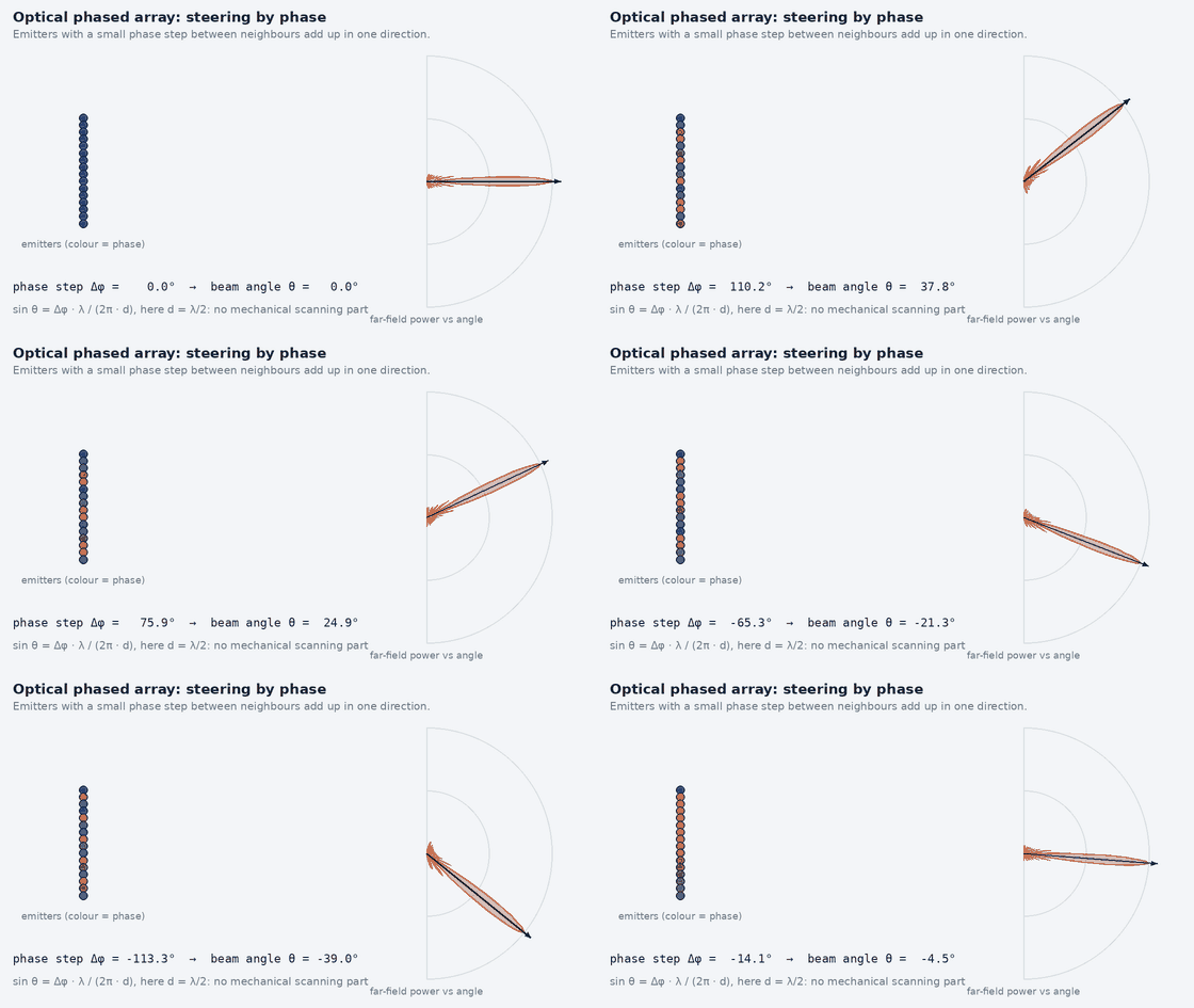
- Phased Arrays – Steering and the Antenna Pattern | An Animated Intro to Phased Arrays · Marshall Bruner · 19:52 (about radio-frequency antenna arrays, not LiDAR: the beam-steering physics (phase differences between elements) is the same idea an optical phased array uses)
No video specifically about optical phased-array LiDAR that I could judge to be an explanation (rather than a product demo) was found; the video above teaches the underlying steering idea for radio waves.
Hybrid / non-repetitive scanning LiDAR
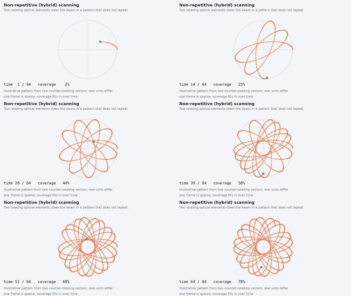
No explanatory video I could judge suitable was found (the search returned product demos). The manufacturer’s own documentation describes its scan pattern.
FMCW (4D) LiDAR
- FMCW vs. ToF LiDAR · SiLC Technologies Inc. · 3:13 (by an FMCW LiDAR maker, so it favours FMCW)
- What is FMCW Radar and why is it useful? · Marshall Bruner · 6:55 (about FMCW radar, not LiDAR: the chirp, beat-frequency and Doppler mathematics is the same, with radio instead of light)
What happens to the scans afterwards
- LiDAR Odometry – 5 Minutes with Cyrill · Cyrill Stachniss · 5:52 (what is done with scans after they are captured)
Time-of-flight and the 2D scanner
A pulsed time-of-flight LiDAR measures the round-trip time t of a light pulse and computes range R = c·t / 2. A 2D scanner sweeps one beam through a plane, so a scan is a list of ranges at known angles. Its important properties are the angular resolution (the angle between neighbouring beams), the scan frequency (how often a full sweep repeats), the field of view (270° models leave a blind sector behind the robot and are easier to mount flush; 360° models need a clear view all round and a mounting that does not block the rear) and the range, which depends on the target’s reflectivity. Accuracy and noise are separate figures from resolution (see the accuracy-versus-precision guide).
- Single plane: anything above or below the scan plane does not exist for the robot: table tops, shelves, wheelchair footrests, the lip of a ramp. A robot tilting on a slope sees the floor or the ceiling instead of the wall.
- Glass and mirrors: the beam passes through clear glass or reflects away from a mirror; the wall appears missing or a ghost appears behind it.
- Dark and low-reflectivity surfaces: less return power means shorter range on that surface than the headline figure.
- Indoor navigation: a 2D scanner plus wheel odometry and an IMU is the proven, low-compute base for scan-matching localisation and costmap obstacle layers on a flat floor.
- Safety-rated versus navigation scanners: a safety laser scanner is a certified component whose detection function, response time and diagnostics are specified for personnel protection. A navigation scanner of similar appearance is not: it has no such certification, and software that stops the robot for obstacles it sees is an ordinary operational safeguard, not a safety function. A single 2D navigation scanner is therefore not automatically sufficient for personnel safety. See Module 18.
Mechanical spinning 3D LiDAR
A spinning 3D LiDAR stacks many emitter–receiver channels at different vertical angles on a rotating assembly (or behind a rotating mirror). The result is 360° horizontal coverage and a vertical field of view of tens of degrees, with a scan pattern of horizontal rings, one per channel. Key quantities: the number of channels, the points per second, the rotation frequency (points per revolution = points per second ÷ rotation rate) and the return modes (single or dual return: strongest, last, or both, which affects how rain, foliage and windows appear).
import math
az_res_deg = 0.2                                    # illustrative horizontal angular step, degrees
step = math.radians(az_res_deg)
for r in (10, 50, 100):                             # range, metres
    spacing = r * step                               # lateral distance between neighbouring beams at that range
    print(r, round(spacing, 3), int(0.5 // spacing)) # spacing (m); beams that land across a 0.5 m wide object
pps, rev_hz = 600_000, 10                           # illustrative point rate (points/s) and rotation rate (Hz)
print(pps // rev_hz)                                # points per revolution
Printed (checked by the site’s tests):
10 0.035 14
50 0.175 2
100 0.349 1
60000
Why density falls with distance: beams leave the sensor at fixed angular steps, so the distance between neighbouring beams at range R is about R × step (step in radians). With an illustrative 0.2° step the spacing is 3.5 cm at 10 m, 17.5 cm at 50 m and 34.9 cm at 100 m: a 0.5 m wide object receives 14 beams per ring at 10 m, 2 at 50 m and 1 at 100 m, and vertical channel spacing grows the same way. Point density per unit area falls with the square of range (both spacings grow). The illustrative 600 000 points per second at 10 Hz is 60 000 points per revolution, spread over the whole sweep.
- Motion distortion: the sweep takes 1/rotation rate seconds (100 ms at 10 Hz); while it runs the robot moves and turns, so points are expressed in a sensor frame that changes during the sweep. Straight walls bend, and a rotating robot smears the scene.
- Deskewing: transform each point to a common time using the motion during the sweep from the IMU or odometry; this needs per-point timestamps and a synchronised clock (see the next section).
- Mechanical reliability and outdoor limits: bearings and motors wear and limit shock and vibration tolerance; rain, spray, fog and dust degrade returns; a dirty window removes a sector.
Deskewing (motion compensation) with a tested example
import math
v, w_deg, T = 5.0, 30.0, 0.1                        # forward speed m/s, yaw rate deg/s, scan duration s
t = T                                               # a point measured at the END of the scan
psi = math.radians(w_deg * t)                       # sensor yaw since scan start
dx = v * t                                          # sensor travel since scan start
x, y = 10.0, 0.0                                    # a wall point seen 10 m ahead, in the sensor frame at time t
xs = math.cos(psi) * x - math.sin(psi) * y + dx     # express it in the sensor frame at scan start
ys = math.sin(psi) * x + math.cos(psi) * y
print(round(xs, 4), round(ys, 4))
print(round(math.hypot(xs - x, ys - y), 2))         # position error if the scan is not deskewed
Printed (checked by the site’s tests):
10.4863 0.5234
0.71
A robot driving at 5 m/s while turning at 30°/s moves 0.5 m and yaws 3° during a 0.1 s sweep. A wall point seen 10 m ahead at the end of the sweep is, in the frame at the start of the sweep, at (10.4863, 0.5234) m: 0.71 m from where an un-deskewed cloud would put it. This is why a slow-looking 10 Hz sensor produces visibly bent walls on a moving vehicle, and why LiDAR–IMU time offset matters (the simulator on the site shows the effect of a few tens of milliseconds).
Non-mechanical-scanning (“solid-state”) LiDAR: four different things
| Type | Principle | Field of view | Range | Resolution and frame rate | Reliability | Optical power and eye safety | Processing |
|---|---|---|---|---|---|---|---|
| Flash | Flood-illuminate the whole scene; a detector array measures arrival time (or phase) per pixel in one exposure | Fixed by the optics | Shorter than scanning types (power per pixel is low) | Pixel count of the array; whole frame at one instant | No scanning mechanism; simple | Eye-safe pulse energy is shared by all pixels, limiting signal per pixel; bright ambient light competes with a weak return | Image-like organised cloud; per-frame processing, no scan distortion |
| MEMS mirror | A micro-mirror oscillates to scan a laser beam | Limited per unit by mirror deflection | Can reach long ranges; mirror size limits the aperture | Set by scan pattern and rate | Small moving part; vibration and shock matter | A concentrated beam allows higher power density within the eye-safety limit | Scan pattern may be non-uniform and need driver handling |
| Optical phased array | Phase control across many emitters steers the beam electronically | Limited by grating lobes and element spacing | Limited so far by optical loss and power per element | Electronically agile in principle | No mechanical scanning element | Power split among elements | Mature products are fewer |
| Hybrid / other | Small rotating or oscillating optics (for example prisms) produce a non-repeating or limited-field scan | Wide for some designs, narrow for others | Model dependent | Dense coverage accumulates over time rather than in one frame | Has moving parts, usually smaller than a spinning head | Model dependent | Algorithms must accept a changing scan pattern |
Flash LiDAR
- Flood illumination: a diffused pulse covers the full field of view at once.
- Detector array: each pixel times its own return, giving a depth image in a single exposure (no sweep, so no motion distortion within the frame).
- Spatial resolution equals the detector array size; it is usually lower than the angular density of a scanning unit.
- Range limitation: the same eye-safe energy is divided among all pixels, so each pixel receives less signal than a scanned beam of equal energy.
- Ambient light: sunlight adds background to every pixel at once and competes with the weak return.
- Eye safety: limits the total pulse energy; this, not the electronics, is the main cap on range.
FMCW LiDAR: range and velocity from a frequency difference
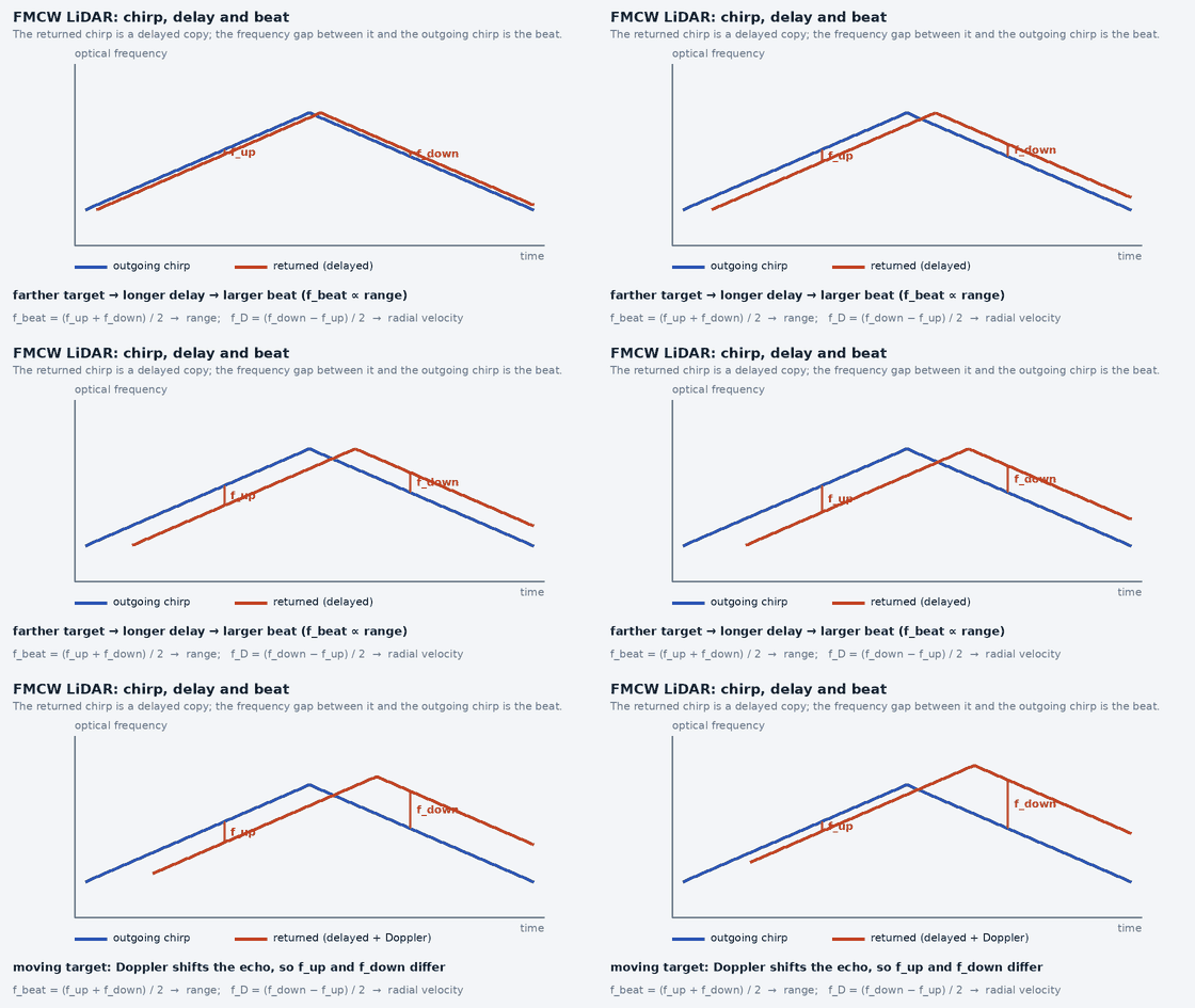
A pulsed sensor times a pulse. A frequency-modulated continuous-wave sensor transmits light whose frequency is swept linearly: a chirp of bandwidth B over duration T, generated by modulating the laser. A copy of the transmitted light is kept as a local oscillator. The returned light, delayed by the round trip τ = 2R/c, is mixed with the local oscillator on the detector (coherent detection); the detector output contains the beat frequency between the two:
f_beat = (B / T) · τ = 2·B·R / (c·T)        so   R = c·T·f_beat / (2·B)
range resolution  ΔR = c / (2·B)
Doppler shift     f_D = 2·v_r / λ                  (v_r = radial velocity)
A moving target adds a Doppler shift to the beat. With a single rising chirp the beat frequency is fbeat ± fD, so range and velocity are ambiguous: a distant stationary target and a nearer approaching one can give the same beat. FMCW sensors resolve this by sweeping the frequency up and then down (a triangular chirp: the two slopes see the Doppler shift with opposite sign) or by processing several chirps together. The two beats are fup = fbeat − fD and fdown = fbeat + fD, so fbeat = (fup + fdown)/2 and fD = (fdown − fup)/2.
c = 3.0e8                                           # speed of light, m/s (rounded)
B, T, lam = 1.0e9, 10e-6, 1550e-9                   # chirp bandwidth (Hz), chirp duration (s), wavelength (m): illustrative values
R, v = 50.0, 10.0                                   # target range (m) and radial velocity (m/s, positive = approaching)
tau = 2 * R / c                                     # round-trip delay
f_beat = (B / T) * tau                              # beat frequency from range alone
f_dopp = 2 * v / lam                                # Doppler shift from radial velocity
print(round(f_beat / 1e6, 1), round(f_dopp / 1e6, 1), round(c / (2 * B), 3))
f_up, f_down = f_beat - f_dopp, f_beat + f_dopp     # triangular chirp: the two slopes see the Doppler shift with opposite sign
f_b = (f_up + f_down) / 2
f_d = (f_down - f_up) / 2
print(round(c * T * f_b / (2 * B), 2), round(f_d * lam / 2, 2))
print(round(10.0 * 0.0, 1))                        # 10 m/s target moving purely sideways: radial component is 0
Printed (checked by the site’s tests):
33.3 12.9 0.15
50.0 10.0
0.0
With illustrative values (1 GHz bandwidth, 10 µs chirp, 1550 nm), a target at 50 m produces a 33.3 MHz beat; a 10 m/s approach adds a 12.9 MHz Doppler shift; the range resolution is 0.15 m; and the triangular-chirp arithmetic recovers 50.0 m and 10.0 m/s. A target moving purely sideways at 10 m/s contributes 0 m/s: the Doppler measurement sees only the component along the beam, so tangential velocity is not measured; it must be inferred from successive frames.
- Ambient light rejection: coherent detection responds to light that is coherent with the local oscillator, so incoherent sunlight does not mix into the beat. Strong ambient light still adds shot noise and can saturate the detector, so FMCW is less affected by sunlight in principle, not immune to it.
- Interference: chirps from another FMCW emitter with overlapping frequencies can produce false beats; pulsed LiDARs can interfere with each other as well. FMCW reduces, but does not remove, interference from other emitters.
- Weather: rain, fog and dust still attenuate and backscatter light at the wavelength used.
- What it adds: a radial velocity for every point in one measurement, useful for separating moving from static objects and for ego-motion; it does not give tangential velocity.
Working range of LiDAR: what the number means
About these figures. The table lists only ranges that were read from a manufacturer’s own page, each with the target reflectivity and conditions it applies to (read 2026-11-05 to 2026-11-06). Models whose range could not be read reliably are not in the table. Generic “typical range by sensor class” lists (for example 10–40 m for 2D and 50–150 m for 3D) circulate without sources; they are not used here, because the sourced figures below show how far a single number can mislead: the same model has very different ranges for a dark and a bright target.
- A LiDAR has no single range. Detection range is quoted for a stated target reflectivity (often 10 % for a dark target and 80 % for a bright one), a detection probability, and sometimes a sunlight level. A dark tyre or black coat is much closer to the 10 % figure than to the bright-target figure.
- Why reflectivity matters (general lidar physics, not from a datasheet). For a target that fills the beam, the returned power falls roughly with the square of distance and is proportional to the target’s reflectivity, so a darker target shortens the distance at which the return still rises above noise. Sunlight adds background light and lowers range further; rain, fog and dust attenuate the beam.
- Minimum range exists too. Many sensors have a blind zone close to the housing (the Livox Mid-360 entry below states one) and 2D scanners list a minimum detection distance.
- Design with the dark-target figure, at the speed you need to stop from: obstacle detection range must exceed stopping distance plus latency, evaluated for the darkest object you must see. Mapping and localization often need less range than obstacle avoidance but need it in every direction.
| Technology | Model | Range, dark-target class (10 % reflectivity) | Range, bright target |
|---|---|---|---|
| 2D scanning LiDAR (time of flight) | Hokuyo UST-10LX | 4 m 10 % diffuse reflectance; detection range 0.06 m to 4 m (maximum detection distance 30 m) · source, read 2026-11-05 | 10 m white Kent sheet; detection range 0.06 m to 10 m · source, read 2026-11-05 |
| 2D scanning LiDAR (time of flight) | Hokuyo UST-20LX | 8 m 10 % diffuse reflectance; detection range 0.06 m to 8 m (maximum detection distance 60 m) · source, read 2026-11-05 | 20 m white Kent sheet; detection range 0.06 m to 20 m · source, read 2026-11-05 |
| 3D mechanical spinning LiDAR | Ouster OS0 (Rev8) | 35 m 10 % Lambertian reflectivity, >90 % detection probability, 100 klx sunlight, 1024 @ 10 Hz mode · source, read 2026-11-05 | 75 m 80 % Lambertian reflectivity, >90 % detection probability, 100 klx sunlight, 1024 @ 10 Hz mode · source, read 2026-11-05 |
| 3D mechanical spinning LiDAR | Ouster OS1 (Rev8) | 90 m 10 % Lambertian reflectivity, >90 % detection probability, 100 klx sunlight, 1024 @ 10 Hz mode · source, read 2026-11-05 | 170 m 80 % Lambertian reflectivity, >90 % detection probability, 100 klx sunlight, 1024 @ 10 Hz mode · source, read 2026-11-05 |
| 3D mechanical spinning LiDAR | Ouster OS1 Max (Rev8) | 200 m 10 % Lambertian reflectivity, >90 % detection probability, 100 klx sunlight, 1024 @ 10 Hz mode · source, read 2026-11-05 | 350 m 80 % Lambertian reflectivity, >90 % detection probability, 100 klx sunlight, 1024 @ 10 Hz mode · source, read 2026-11-05 |
| 3D mechanical spinning LiDAR | Ouster OS2 (Rev7) | 200 m 10 % Lambertian reflectivity, >90 % detection probability, 100 klx sunlight, 1024 @ 10 Hz mode · source, read 2026-11-05 | 350 m 80 % Lambertian reflectivity, >90 % detection probability, 100 klx sunlight, 1024 @ 10 Hz mode · source, read 2026-11-05 |
| 3D mechanical spinning LiDAR | Ouster OSDome (Rev8) | 20 m 10 % Lambertian reflectivity, >90 % detection probability, 100 klx sunlight, 1024 @ 10 Hz mode · source, read 2026-11-05 | 45 m 80 % Lambertian reflectivity, >90 % detection probability, 100 klx sunlight, 1024 @ 10 Hz mode · source, read 2026-11-05 |
| 3D mechanical spinning LiDAR | Hesai Pandar128 | 200 m 10 % reflectivity (“ranging capability”), typical value under the manufacturer’s test conditions · source, read 2026-11-05 | Not stated for this model in the source read |
| 3D hybrid / non-repetitive scanning LiDAR | Livox Mid-360 | 40 m 10 % reflectivity, at 100 klx; blind zone 0.1 m · source, read 2026-11-05 | 70 m 80 % reflectivity, at 100 klx · source, read 2026-11-05 |
Reading the table: the 2D scanners (Hokuyo UST series) are specified for a few metres on a dark target and about two and a half times that on a white one, with a separate, larger “maximum detection distance” in the text; the 3D spinning units from Ouster span from tens of metres (dome and short-range models) to hundreds of metres on a bright target; the Livox Mid-360 sits in between. Sensors of the same class differ by an order of magnitude, so pick from the exact model’s datasheet, not from a class average. Radar, ultrasonic, camera, thermal and GNSS ranges are outside this section: the camera guide has sourced depth ranges for the depth cameras read there.
Real-World LiDAR Products and Manufacturer Comparison
Status of this section (read 2026-11-05 and 2026-11-06). Specifications for 10 models (Ouster OS0, OS1, OS1 Max, OS2 and OSDome, Livox Mid-360, Hokuyo UST-10LX and UST-20LX, Hesai Pandar128 and the Velodyne VLP-16 from its user manual) were read from the manufacturer’s own datasheet or specification page; each figure below shows its unit, the operating mode and target reflectivity it applies to, and a link to the source with the date read. For the other 6 products the manufacturer’s documentation could not be used in this build (site blocked, no specification text in the static page, or no datasheet found), so no specification is shown for them: the cards give only the vendor’s general category and a link to the manufacturer’s site. Photographs: the Ouster, Hesai, Velodyne, Blickfeld and Aeva cards show a photograph from the manufacturer’s own page (the Velodyne one from the Ouster-hosted page), with a credit and a link to that page; the Ouster images were supplied by the site owner and the others were saved and resized for this site. Reuse permission for these images has not been verified by this build and should be confirmed with each company. The other products show a labelled placeholder because no photograph was available. Not used on purpose: the Ouster-hosted Velodyne page lists a summary (200 m, 16 to 32 channels) that appears to describe the family, not the VLP-16, and the Blickfeld and Aeva pages had no usable specification text (Aeva states a long detection range for dynamic objects with no reflectivity condition).
Reading the figures: keep four kinds apart: manufacturer specifications (guaranteed limits), typical performance (what a unit usually does), best-case performance (for example range on a highly reflective target) and independently measured performance. Everything in these cards is a manufacturer statement; none is independently measured. Range is shown at 10 % reflectivity as the comparable column, with the bright-target figure beside it: do not compare a 10 % range with an 80 % range. A Hokuyo “white Kent sheet” range and an Ouster “80 % Lambertian” range are both bright-target figures but not the same target, and Ouster’s ranges also state a 100 klx sunlight and a 1024 @ 10 Hz mode condition, which differ from a different manufacturer’s test conditions.
SICK TiM series
Technology: 2D scanning LiDAR (time of flight) (category from the manufacturer’s general positioning; not verified against its documentation in this build)
Compact 2D scanning LiDAR family for industrial and mobile-robot navigation and object detection. Choose the exact TiM model: variants differ in range, field of view and interface.
- Detection range (10 % reflectivity class)
- Not yet verified in this build
- Detection range (bright target)
- Not yet verified in this build
- Field of view
- Not yet verified in this build
- Range accuracy / precision
- Not yet verified in this build
- Resolution / channels
- Not yet verified in this build
- Update rate
- Not yet verified in this build
- Point rate
- Not yet verified in this build
- Interface
- Not yet verified in this build
Manufacturer site · Product page: link not verified · Datasheet: link not verified
Hokuyo UST-10LX
Technology: 2D scanning LiDAR (time of flight) (as described in the manufacturer’s documentation)
Compact 2D scanning LiDAR for mobile robots. A navigation sensor, not a safety-rated function.
- Detection range (10 % reflectivity class)
- 4 m 10 % diffuse reflectance; detection range 0.06 m to 4 m (maximum detection distance 30 m) · manufacturer specification page, read 2026-11-05
- Detection range (bright target)
- 10 m white Kent sheet; detection range 0.06 m to 10 m · manufacturer specification page, read 2026-11-05
- Field of view
- 270 ° scan angle (horizontal, single plane) · manufacturer specification page, read 2026-11-05
- Range accuracy / precision
- ±40 mm manufacturer’s table, footnote *1 gives the conditions: read the datasheet before relying on it · manufacturer specification page, read 2026-11-05
- Resolution / channels
- 0.25 ° angular resolution of the UST-10LX (the -H01 variant is listed at 0.125°) · manufacturer specification page, read 2026-11-05
- Update rate
- 25 ms per scan scan speed, motor speed 2400 rpm (about 40 Hz) · manufacturer specification page, read 2026-11-05
- Point rate
- Not yet verified in this build
- Interface
- Ethernet 100BASE-TX as listed in the specification table · manufacturer specification page, read 2026-11-05
Manufacturer site · Official product page · Specification page
Hokuyo UST-20LX
Technology: 2D scanning LiDAR (time of flight) (as described in the manufacturer’s documentation)
Longer-range member of the same 2D scanning family as the UST-10LX; same field of view and scan speed, larger detection range. Not a safety-rated function.
- Detection range (10 % reflectivity class)
- 8 m 10 % diffuse reflectance; detection range 0.06 m to 8 m (maximum detection distance 60 m) · manufacturer specification page, read 2026-11-05
- Detection range (bright target)
- 20 m white Kent sheet; detection range 0.06 m to 20 m · manufacturer specification page, read 2026-11-05
- Field of view
- 270 ° scan angle (horizontal, single plane) · manufacturer specification page, read 2026-11-05
- Range accuracy / precision
- ±40 mm manufacturer’s table, footnote *1 gives the conditions: read the datasheet before relying on it · manufacturer specification page, read 2026-11-05
- Resolution / channels
- 0.25 ° angular resolution of the UST-20LX (the -H01 variant is listed at 0.125°) · manufacturer specification page, read 2026-11-05
- Update rate
- 25 ms per scan scan speed, motor speed 2400 rpm (about 40 Hz) · manufacturer specification page, read 2026-11-05
- Point rate
- Not yet verified in this build
- Interface
- Ethernet 100BASE-TX as listed in the specification table · manufacturer specification page, read 2026-11-05
Manufacturer site · Official product page · Specification page
OMRON OS32C
Technology: 2D safety laser scanner (safety-rated) (category from the manufacturer’s general positioning; not verified against its documentation in this build)
Safety laser scanner for protecting people around machines and vehicles. It is a certified safety component, which is different from a navigation scanner of similar appearance.
- Detection range (10 % reflectivity class)
- Not yet verified in this build
- Detection range (bright target)
- Not yet verified in this build
- Field of view
- Not yet verified in this build
- Range accuracy / precision
- Not yet verified in this build
- Resolution / channels
- Not yet verified in this build
- Update rate
- Not yet verified in this build
- Point rate
- Not yet verified in this build
- Interface
- Not yet verified in this build
Manufacturer site · Product page: link not verified · Datasheet: link not verified
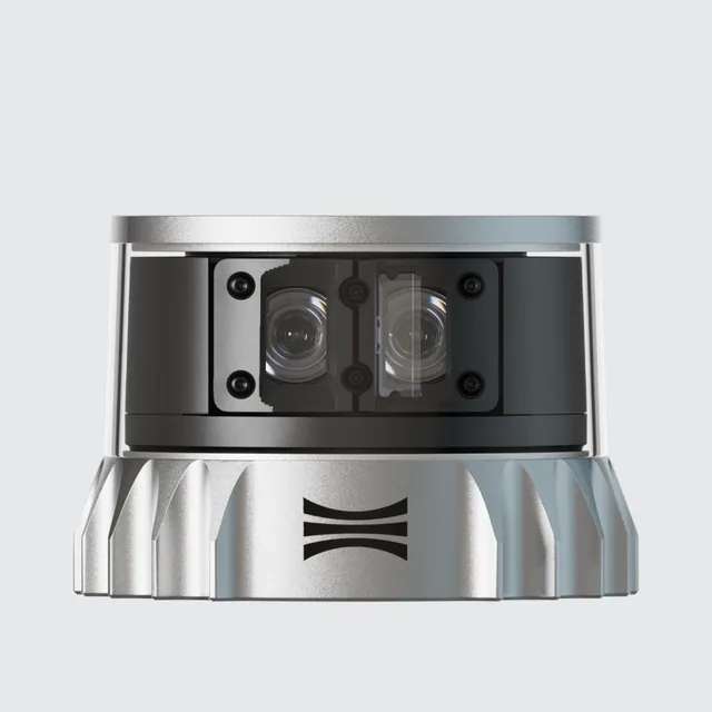
Ouster OS0 (Rev8)
Technology: 3D mechanical spinning LiDAR (as described in the manufacturer’s documentation)
Wide field-of-view spinning 3D LiDAR for AMRs, AGVs and other close-range robotics, per the manufacturer’s datasheet.
- Detection range (10 % reflectivity class)
- 35 m 10 % Lambertian reflectivity, >90 % detection probability, 100 klx sunlight, 1024 @ 10 Hz mode · datasheet, read 2026-11-05
- Detection range (bright target)
- 75 m 80 % Lambertian reflectivity, >90 % detection probability, 100 klx sunlight, 1024 @ 10 Hz mode · datasheet, read 2026-11-05
- Field of view
- 360 ° horizontal; vertical 90.0° (+45.0° to −45.0°) · datasheet, read 2026-11-05
- Range accuracy / precision
- ±1.25 (Lambertian), ±2.5 (retroreflective) cm typical, targets beyond 1 m, 1024 @ 10 Hz mode · datasheet, read 2026-11-05
- Resolution / channels
- 32, 64 or 128 channels; 512–4096 columns configurable; angular sampling accuracy ±0.01° vertical and horizontal · datasheet, read 2026-11-05
- Update rate
- 5, 10, 15, 20, 30 or 40 Hz rotation rate configurable, mode dependent · datasheet, read 2026-11-05
- Point rate
- 10,485,760 points/s maximum, highest-resolution mode · datasheet, read 2026-11-05
- Interface
- UDP over gigabit Ethernet (1000BASE-T) lidar output; IMU output also UDP over 1000BASE-T · datasheet, read 2026-11-05
Ouster OS1 (Rev8)
Technology: 3D mechanical spinning LiDAR (as described in the manufacturer’s documentation)
Mid-range spinning 3D LiDAR with a balanced field of view, positioned by the manufacturer for robotics, mapping and automation; native colour RGB-D point cloud in Rev8.
- Detection range (10 % reflectivity class)
- 90 m 10 % Lambertian reflectivity, >90 % detection probability, 100 klx sunlight, 1024 @ 10 Hz mode · datasheet, read 2026-11-05
- Detection range (bright target)
- 170 m 80 % Lambertian reflectivity, >90 % detection probability, 100 klx sunlight, 1024 @ 10 Hz mode · datasheet, read 2026-11-05
- Field of view
- 360 ° horizontal; vertical 44.0° (+22.0° to −22.0°) · datasheet, read 2026-11-05
- Range accuracy / precision
- ±1.25 (Lambertian), ±2.5 (retroreflective) cm typical, targets beyond 1 m, 1024 @ 10 Hz mode · datasheet, read 2026-11-05
- Resolution / channels
- 32, 64 or 128 channels; 512–4096 columns configurable; angular sampling accuracy ±0.01° vertical and horizontal · datasheet, read 2026-11-05
- Update rate
- 5, 10, 15, 20, 30 or 40 Hz rotation rate configurable, mode dependent · datasheet, read 2026-11-05
- Point rate
- 10,485,760 points/s maximum, highest-resolution mode · datasheet, read 2026-11-05
- Interface
- UDP over gigabit Ethernet (1000BASE-T) lidar output; IMU output also UDP over 1000BASE-T · datasheet, read 2026-11-05
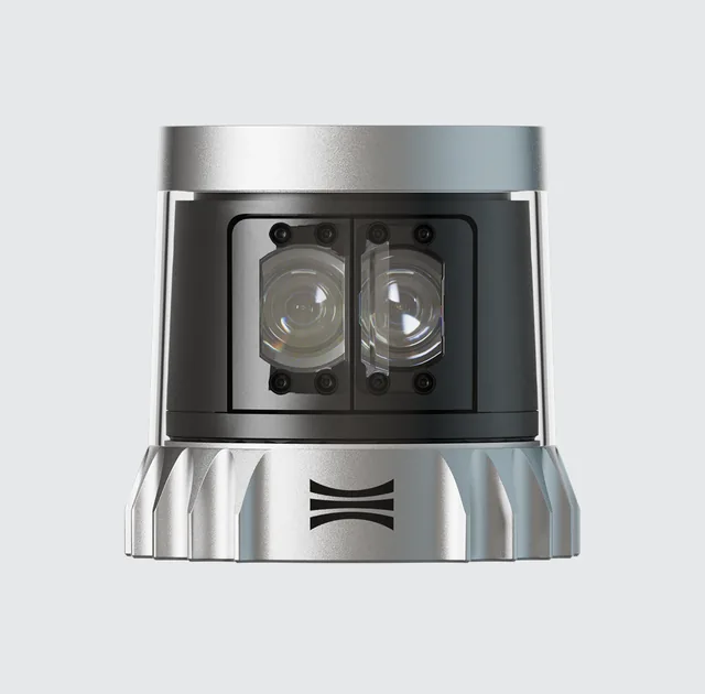
Ouster OS1 Max (Rev8)
Technology: 3D mechanical spinning LiDAR (as described in the manufacturer’s documentation)
Flagship long-range member of the Rev8 OS series with the highest channel count of the family, positioned by the manufacturer for off-highway vehicles, autonomous vehicles and mapping, per its datasheet.
- Detection range (10 % reflectivity class)
- 200 m 10 % Lambertian reflectivity, >90 % detection probability, 100 klx sunlight, 1024 @ 10 Hz mode · datasheet, read 2026-11-05
- Detection range (bright target)
- 350 m 80 % Lambertian reflectivity, >90 % detection probability, 100 klx sunlight, 1024 @ 10 Hz mode · datasheet, read 2026-11-05
- Field of view
- 360 ° horizontal; vertical 43.9° (+21.95° to −21.95°) · datasheet, read 2026-11-05
- Range accuracy / precision
- ±1.25 (Lambertian), ±2.5 (retroreflective) cm typical, targets beyond 1 m, 1024 @ 10 Hz mode · datasheet, read 2026-11-05
- Resolution / channels
- 64, 128 or 256 channels; 512–4096 columns configurable; angular sampling accuracy ±0.01° vertical and horizontal · datasheet, read 2026-11-05
- Update rate
- 5, 10, 15, 20, 30 or 40 Hz rotation rate configurable, mode dependent · datasheet, read 2026-11-05
- Point rate
- 10,485,760 points/s maximum, highest-resolution mode · datasheet, read 2026-11-05
- Interface
- UDP over gigabit Ethernet (1000BASE-T) lidar output; IMU output also UDP over 1000BASE-T · datasheet, read 2026-11-05
Ouster OS2 (Rev7)
Technology: 3D mechanical spinning LiDAR (as described in the manufacturer’s documentation)
Long-range spinning 3D LiDAR with a narrower vertical field of view, for vehicles and outdoor robots, per the manufacturer’s Rev7 datasheet (the latest OS2 sheet listed on the manufacturer’s downloads page when read).
- Detection range (10 % reflectivity class)
- 200 m 10 % Lambertian reflectivity, >90 % detection probability, 100 klx sunlight, 1024 @ 10 Hz mode · datasheet, read 2026-11-05
- Detection range (bright target)
- 350 m 80 % Lambertian reflectivity, >90 % detection probability, 100 klx sunlight, 1024 @ 10 Hz mode · datasheet, read 2026-11-05
- Field of view
- 360 ° horizontal; vertical 22.5° (+11.25° to −11.25°) · datasheet, read 2026-11-05
- Range accuracy / precision
- ±2.5 (Lambertian), ±5 (retroreflective) cm typical, targets beyond 1 m, 1024 @ 10 Hz mode · datasheet, read 2026-11-05
- Resolution / channels
- 32, 64 or 128 channels; 512, 1024 or 2048 columns configurable; angular sampling accuracy ±0.01° vertical and horizontal · datasheet, read 2026-11-05
- Update rate
- 10 or 20 Hz rotation rate configurable · datasheet, read 2026-11-05
- Point rate
- 2,621,440 points/s maximum, 128-channel sensor · datasheet, read 2026-11-05
- Interface
- UDP over gigabit Ethernet (1000BASE-T) lidar output · datasheet, read 2026-11-05
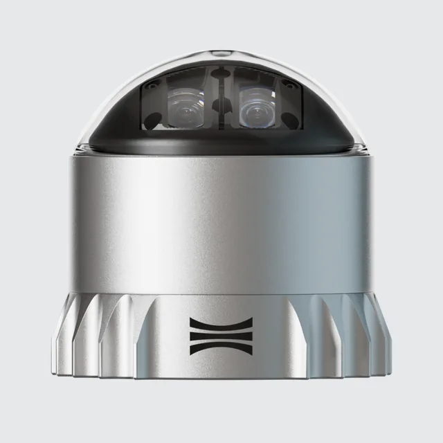
Ouster OSDome (Rev8)
Technology: 3D mechanical spinning LiDAR (as described in the manufacturer’s documentation)
Short-range hemispherical spinning-class 3D LiDAR with a 180° vertical field of view, positioned by the manufacturer for indoor people tracking and near-range detection on robots and vehicles. The datasheet uses the same rotation-rate and column terminology as the OS family: read it for the mechanical design.
- Detection range (10 % reflectivity class)
- 20 m 10 % Lambertian reflectivity, >90 % detection probability, 100 klx sunlight, 1024 @ 10 Hz mode · datasheet, read 2026-11-05
- Detection range (bright target)
- 45 m 80 % Lambertian reflectivity, >90 % detection probability, 100 klx sunlight, 1024 @ 10 Hz mode · datasheet, read 2026-11-05
- Field of view
- 360 ° horizontal; vertical 180.0° (hemispherical) · datasheet, read 2026-11-05
- Range accuracy / precision
- ±1.25 (Lambertian), ±2.5 (retroreflective) cm typical, targets beyond 1 m, 1024 @ 10 Hz mode · datasheet, read 2026-11-05
- Resolution / channels
- 32, 64 or 128 channels; 512–4096 columns configurable; angular sampling accuracy ±0.01° vertical and horizontal · datasheet, read 2026-11-05
- Update rate
- 5, 10, 15, 20, 30 or 40 Hz rotation rate configurable, mode dependent · datasheet, read 2026-11-05
- Point rate
- 10,485,760 points/s maximum, highest-resolution mode · datasheet, read 2026-11-05
- Interface
- UDP over gigabit Ethernet (1000BASE-T) lidar output; IMU output also UDP over 1000BASE-T · datasheet, read 2026-11-05
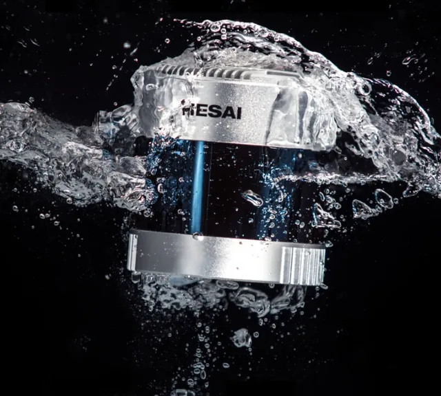
Hesai Pandar128
Technology: 3D mechanical spinning LiDAR (as described in the manufacturer’s documentation)
Mechanical spinning 128-channel 3D LiDAR from Hesai’s Pandar line, described on its page as auto-grade, high-performance and long-range. The manufacturer’s page says its values are typical under specific test conditions.
- Detection range (10 % reflectivity class)
- 200 m 10 % reflectivity (“ranging capability”), typical value under the manufacturer’s test conditions · manufacturer specification page, read 2026-11-05
- Detection range (bright target)
- Not yet verified in this build
- Field of view
- 360 ° horizontal; vertical field of view 40°, stated as “360° x 40°” · manufacturer specification page, read 2026-11-05
- Range accuracy / precision
- Not yet verified in this build
- Resolution / channels
- 0.1° (H) × 0.125° (V) angular resolution as stated; the page title says 128-channel; the horizontal figure is given at 10 Hz · manufacturer specification page, read 2026-11-05
- Update rate
- Not yet verified in this build
- Point rate
- 3,456,000 points/s single return; the page gives 6,912,000 points/s in dual return · manufacturer specification page, read 2026-11-05
- Interface
- Not yet verified in this build
Manufacturer site · Official product page · Specification page
RoboSense RS series
Technology: 3D mechanical spinning LiDAR (category from the manufacturer’s general positioning; not verified against its documentation in this build)
Spinning multi-channel 3D LiDAR family. The manufacturer’s other series use different architectures: take the architecture from the exact model’s datasheet.
- Detection range (10 % reflectivity class)
- Not yet verified in this build
- Detection range (bright target)
- Not yet verified in this build
- Field of view
- Not yet verified in this build
- Range accuracy / precision
- Not yet verified in this build
- Resolution / channels
- Not yet verified in this build
- Update rate
- Not yet verified in this build
- Point rate
- Not yet verified in this build
- Interface
- Not yet verified in this build
Manufacturer site · Product page: link not verified · Datasheet: link not verified
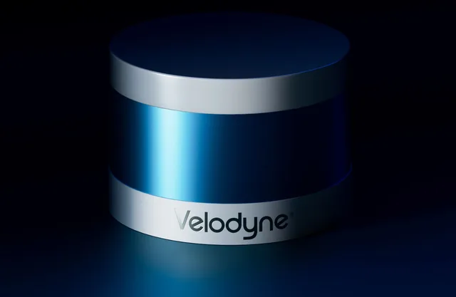
Velodyne VLP-16 Puck
Technology: 3D mechanical spinning LiDAR (as described in the manufacturer’s documentation)
A widely deployed spinning 3D LiDAR, important historically for robotics research and datasets. The velodynelidar.com website now redirects to Ouster, which hosts the Velodyne downloads; the user manual used here is Rev F and its pages carry a DRAFT mark. Check current availability and support status with the manufacturer. The Ouster-hosted product page shows a summary of range and channel counts that appears to describe the Velodyne family rather than this sensor, so it was not used.
- Detection range (10 % reflectivity class)
- Not yet verified in this build
- Detection range (bright target)
- Not yet verified in this build
- Field of view
- Not yet verified in this build
- Range accuracy / precision
- Not yet verified in this build
- Resolution / channels
- 16 lasers (channels) user manual: all 16 lasers fire every 55.296 µs; vertical angles run from −15° to +15° (Table 9-1) · datasheet, read 2026-11-05
- Update rate
- 5 to 20 Hz motor rotation of 300 to 1200 RPM in steps of 60 RPM (manual section 8.3); one rotation is one frame · datasheet, read 2026-11-05
- Point rate
- 289,344 points/s maximum laser measurements per second in single return mode; 578,688 in dual return (manual section 8.2.4) · datasheet, read 2026-11-05
- Interface
- Ethernet the manual recommends at least a 100 Mbps Ethernet adapter · datasheet, read 2026-11-05
Manufacturer site · Official product page · Specification page
Livox Mid-360
Technology: 3D hybrid / non-repetitive scanning LiDAR (as described in the manufacturer’s documentation)
Compact 3D LiDAR with a non-repetitive scanning pattern, positioned by the vendor for robotics. Point density builds up over integration time rather than appearing in one frame.
- Detection range (10 % reflectivity class)
- 40 m 10 % reflectivity, at 100 klx; blind zone 0.1 m · manufacturer specification page, read 2026-11-05
- Detection range (bright target)
- 70 m 80 % reflectivity, at 100 klx · manufacturer specification page, read 2026-11-05
- Field of view
- 360 ° horizontal; vertical −7° to 52° · manufacturer specification page, read 2026-11-05
- Range accuracy / precision
- ≤ 2 cm range precision (1σ) at 10 m, 80 % reflectivity target, 25 °C; ≤ 3 cm at 0.2 m, same conditions · manufacturer specification page, read 2026-11-05
- Resolution / channels
- Not specified as channels non-repetitive scan pattern; the manufacturer specifies point and frame rate instead · manufacturer specification page, read 2026-11-05
- Update rate
- 10 Hz frame rate typical · manufacturer specification page, read 2026-11-05
- Point rate
- 200,000 points/s first return · manufacturer specification page, read 2026-11-05
- Interface
- 100BASE-TX Ethernet data port; time synchronisation by IEEE 1588-2008 (PTPv2) or GPS; built-in IMU · manufacturer specification page, read 2026-11-05
Manufacturer site · Official product page · Specification page
Innoviz InnovizTwo
Technology: 3D MEMS-mirror scanning LiDAR (category from the manufacturer’s general positioning; not verified against its documentation in this build)
Automotive-grade 3D LiDAR positioned by the vendor as MEMS-based solid-state, for ADAS and autonomous driving.
- Detection range (10 % reflectivity class)
- Not yet verified in this build
- Detection range (bright target)
- Not yet verified in this build
- Field of view
- Not yet verified in this build
- Range accuracy / precision
- Not yet verified in this build
- Resolution / channels
- Not yet verified in this build
- Update rate
- Not yet verified in this build
- Point rate
- Not yet verified in this build
- Interface
- Not yet verified in this build
Manufacturer site · Product page: link not verified · Datasheet: link not verified
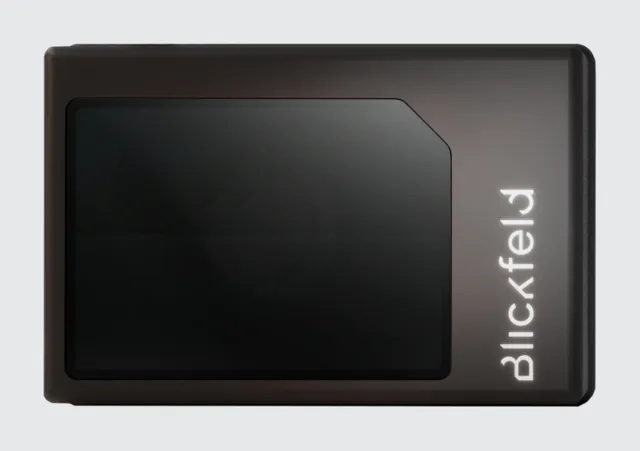
Blickfeld Qb2
Technology: 3D MEMS-mirror scanning LiDAR (category from the manufacturer’s general positioning; not verified against its documentation in this build)
Smart 3D LiDAR with on-device processing, from Blickfeld’s family that the vendor positions as MEMS-mirror scanning for industrial, smart-infrastructure and robotics use. Its page text could not be read as plain text in this build, so no specification is shown.
- Detection range (10 % reflectivity class)
- Not yet verified in this build
- Detection range (bright target)
- Not yet verified in this build
- Field of view
- Not yet verified in this build
- Range accuracy / precision
- Not yet verified in this build
- Resolution / channels
- Not yet verified in this build
- Update rate
- Not yet verified in this build
- Point rate
- Not yet verified in this build
- Interface
- Not yet verified in this build
Manufacturer site · Product page: link not verified · Datasheet: link not verified
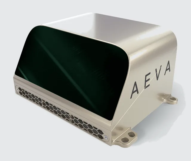
Aeva Aeries II
Technology: 3D FMCW (4D) LiDAR (category from the manufacturer’s general positioning; not verified against its documentation in this build)
Frequency-modulated continuous-wave ("4D") LiDAR that reports radial velocity per point in addition to range. The product page describes a LiDAR-on-chip design with multiple fields of view; it states an ultra-long detection range for dynamic objects without a reflectivity condition, so no range figure is shown here. Not a conventional pulsed time-of-flight sensor.
- Detection range (10 % reflectivity class)
- Not yet verified in this build
- Detection range (bright target)
- Not yet verified in this build
- Field of view
- Not yet verified in this build
- Range accuracy / precision
- Not yet verified in this build
- Resolution / channels
- Not yet verified in this build
- Update rate
- Not yet verified in this build
- Point rate
- Not yet verified in this build
- Interface
- Not yet verified in this build
Manufacturer site · Official product page · Datasheet: link not verified
No product prices are shown: reliable public pricing was not available, and prices are never estimated here. The Sensor Selection Calculator’s cost scale is a relative class for sensor types, not a product price.
Manufacturer comparison table
Grouped by technology so that different architectures are not compared as if equivalent. Range is the 10 %-reflectivity figure; the condition under each value says what it applies to. Cells that read “Not yet verified” have no usable manufacturer source in this build.
| Technology | Manufacturer | Model | Range (m, 10 % reflectivity) | FOV (°) | Accuracy | Resolution / channels | Update rate | Interface | Datasheet |
|---|---|---|---|---|---|---|---|---|---|
| 2D scanning LiDAR (time of flight) | SICK | TiM series | Not yet verified in this build | Not yet verified in this build | Not yet verified in this build | Not yet verified in this build | Not yet verified in this build | Not yet verified in this build | link not verified |
| 2D scanning LiDAR (time of flight) | Hokuyo | UST-10LX | 4 m 10 % diffuse reflectance; detection range 0.06 m to 4 m (maximum detection distance 30 m) · manufacturer specification page, read 2026-11-05 | 270 ° scan angle (horizontal, single plane) · manufacturer specification page, read 2026-11-05 | ±40 mm manufacturer’s table, footnote *1 gives the conditions: read the datasheet before relying on it · manufacturer specification page, read 2026-11-05 | 0.25 ° angular resolution of the UST-10LX (the -H01 variant is listed at 0.125°) · manufacturer specification page, read 2026-11-05 | 25 ms per scan scan speed, motor speed 2400 rpm (about 40 Hz) · manufacturer specification page, read 2026-11-05 | Ethernet 100BASE-TX as listed in the specification table · manufacturer specification page, read 2026-11-05 | spec page |
| 2D scanning LiDAR (time of flight) | Hokuyo | UST-20LX | 8 m 10 % diffuse reflectance; detection range 0.06 m to 8 m (maximum detection distance 60 m) · manufacturer specification page, read 2026-11-05 | 270 ° scan angle (horizontal, single plane) · manufacturer specification page, read 2026-11-05 | ±40 mm manufacturer’s table, footnote *1 gives the conditions: read the datasheet before relying on it · manufacturer specification page, read 2026-11-05 | 0.25 ° angular resolution of the UST-20LX (the -H01 variant is listed at 0.125°) · manufacturer specification page, read 2026-11-05 | 25 ms per scan scan speed, motor speed 2400 rpm (about 40 Hz) · manufacturer specification page, read 2026-11-05 | Ethernet 100BASE-TX as listed in the specification table · manufacturer specification page, read 2026-11-05 | spec page |
| 2D safety laser scanner (safety-rated) | OMRON | OS32C | Not yet verified in this build | Not yet verified in this build | Not yet verified in this build | Not yet verified in this build | Not yet verified in this build | Not yet verified in this build | link not verified |
| 3D mechanical spinning LiDAR | Ouster | OS0 (Rev8) | 35 m 10 % Lambertian reflectivity, >90 % detection probability, 100 klx sunlight, 1024 @ 10 Hz mode · datasheet, read 2026-11-05 | 360 ° horizontal; vertical 90.0° (+45.0° to −45.0°) · datasheet, read 2026-11-05 | ±1.25 (Lambertian), ±2.5 (retroreflective) cm typical, targets beyond 1 m, 1024 @ 10 Hz mode · datasheet, read 2026-11-05 | 32, 64 or 128 channels; 512–4096 columns configurable; angular sampling accuracy ±0.01° vertical and horizontal · datasheet, read 2026-11-05 | 5, 10, 15, 20, 30 or 40 Hz rotation rate configurable, mode dependent · datasheet, read 2026-11-05 | UDP over gigabit Ethernet (1000BASE-T) lidar output; IMU output also UDP over 1000BASE-T · datasheet, read 2026-11-05 | |
| 3D mechanical spinning LiDAR | Ouster | OS1 (Rev8) | 90 m 10 % Lambertian reflectivity, >90 % detection probability, 100 klx sunlight, 1024 @ 10 Hz mode · datasheet, read 2026-11-05 | 360 ° horizontal; vertical 44.0° (+22.0° to −22.0°) · datasheet, read 2026-11-05 | ±1.25 (Lambertian), ±2.5 (retroreflective) cm typical, targets beyond 1 m, 1024 @ 10 Hz mode · datasheet, read 2026-11-05 | 32, 64 or 128 channels; 512–4096 columns configurable; angular sampling accuracy ±0.01° vertical and horizontal · datasheet, read 2026-11-05 | 5, 10, 15, 20, 30 or 40 Hz rotation rate configurable, mode dependent · datasheet, read 2026-11-05 | UDP over gigabit Ethernet (1000BASE-T) lidar output; IMU output also UDP over 1000BASE-T · datasheet, read 2026-11-05 | |
| 3D mechanical spinning LiDAR | Ouster | OS1 Max (Rev8) | 200 m 10 % Lambertian reflectivity, >90 % detection probability, 100 klx sunlight, 1024 @ 10 Hz mode · datasheet, read 2026-11-05 | 360 ° horizontal; vertical 43.9° (+21.95° to −21.95°) · datasheet, read 2026-11-05 | ±1.25 (Lambertian), ±2.5 (retroreflective) cm typical, targets beyond 1 m, 1024 @ 10 Hz mode · datasheet, read 2026-11-05 | 64, 128 or 256 channels; 512–4096 columns configurable; angular sampling accuracy ±0.01° vertical and horizontal · datasheet, read 2026-11-05 | 5, 10, 15, 20, 30 or 40 Hz rotation rate configurable, mode dependent · datasheet, read 2026-11-05 | UDP over gigabit Ethernet (1000BASE-T) lidar output; IMU output also UDP over 1000BASE-T · datasheet, read 2026-11-05 | |
| 3D mechanical spinning LiDAR | Ouster | OS2 (Rev7) | 200 m 10 % Lambertian reflectivity, >90 % detection probability, 100 klx sunlight, 1024 @ 10 Hz mode · datasheet, read 2026-11-05 | 360 ° horizontal; vertical 22.5° (+11.25° to −11.25°) · datasheet, read 2026-11-05 | ±2.5 (Lambertian), ±5 (retroreflective) cm typical, targets beyond 1 m, 1024 @ 10 Hz mode · datasheet, read 2026-11-05 | 32, 64 or 128 channels; 512, 1024 or 2048 columns configurable; angular sampling accuracy ±0.01° vertical and horizontal · datasheet, read 2026-11-05 | 10 or 20 Hz rotation rate configurable · datasheet, read 2026-11-05 | UDP over gigabit Ethernet (1000BASE-T) lidar output · datasheet, read 2026-11-05 | |
| 3D mechanical spinning LiDAR | Ouster | OSDome (Rev8) | 20 m 10 % Lambertian reflectivity, >90 % detection probability, 100 klx sunlight, 1024 @ 10 Hz mode · datasheet, read 2026-11-05 | 360 ° horizontal; vertical 180.0° (hemispherical) · datasheet, read 2026-11-05 | ±1.25 (Lambertian), ±2.5 (retroreflective) cm typical, targets beyond 1 m, 1024 @ 10 Hz mode · datasheet, read 2026-11-05 | 32, 64 or 128 channels; 512–4096 columns configurable; angular sampling accuracy ±0.01° vertical and horizontal · datasheet, read 2026-11-05 | 5, 10, 15, 20, 30 or 40 Hz rotation rate configurable, mode dependent · datasheet, read 2026-11-05 | UDP over gigabit Ethernet (1000BASE-T) lidar output; IMU output also UDP over 1000BASE-T · datasheet, read 2026-11-05 | |
| 3D mechanical spinning LiDAR | Hesai | Pandar128 | 200 m 10 % reflectivity (“ranging capability”), typical value under the manufacturer’s test conditions · manufacturer specification page, read 2026-11-05 | 360 ° horizontal; vertical field of view 40°, stated as “360° x 40°” · manufacturer specification page, read 2026-11-05 | Not yet verified in this build | 0.1° (H) × 0.125° (V) angular resolution as stated; the page title says 128-channel; the horizontal figure is given at 10 Hz · manufacturer specification page, read 2026-11-05 | Not yet verified in this build | Not yet verified in this build | spec page |
| 3D mechanical spinning LiDAR | RoboSense | RS series | Not yet verified in this build | Not yet verified in this build | Not yet verified in this build | Not yet verified in this build | Not yet verified in this build | Not yet verified in this build | link not verified |
| 3D mechanical spinning LiDAR | Velodyne | VLP-16 Puck | Not yet verified in this build | Not yet verified in this build | Not yet verified in this build | 16 lasers (channels) user manual: all 16 lasers fire every 55.296 µs; vertical angles run from −15° to +15° (Table 9-1) · datasheet, read 2026-11-05 | 5 to 20 Hz motor rotation of 300 to 1200 RPM in steps of 60 RPM (manual section 8.3); one rotation is one frame · datasheet, read 2026-11-05 | Ethernet the manual recommends at least a 100 Mbps Ethernet adapter · datasheet, read 2026-11-05 | spec page |
| 3D MEMS-mirror scanning LiDAR | Innoviz | InnovizTwo | Not yet verified in this build | Not yet verified in this build | Not yet verified in this build | Not yet verified in this build | Not yet verified in this build | Not yet verified in this build | link not verified |
| 3D MEMS-mirror scanning LiDAR | Blickfeld | Qb2 | Not yet verified in this build | Not yet verified in this build | Not yet verified in this build | Not yet verified in this build | Not yet verified in this build | Not yet verified in this build | link not verified |
| 3D hybrid / non-repetitive scanning LiDAR | Livox | Mid-360 | 40 m 10 % reflectivity, at 100 klx; blind zone 0.1 m · manufacturer specification page, read 2026-11-05 | 360 ° horizontal; vertical −7° to 52° · manufacturer specification page, read 2026-11-05 | ≤ 2 cm range precision (1σ) at 10 m, 80 % reflectivity target, 25 °C; ≤ 3 cm at 0.2 m, same conditions · manufacturer specification page, read 2026-11-05 | Not specified as channels non-repetitive scan pattern; the manufacturer specifies point and frame rate instead · manufacturer specification page, read 2026-11-05 | 10 Hz frame rate typical · manufacturer specification page, read 2026-11-05 | 100BASE-TX Ethernet data port; time synchronisation by IEEE 1588-2008 (PTPv2) or GPS; built-in IMU · manufacturer specification page, read 2026-11-05 | spec page |
| 3D FMCW (4D) LiDAR | Aeva | Aeries II | Not yet verified in this build | Not yet verified in this build | Not yet verified in this build | Not yet verified in this build | Not yet verified in this build | Not yet verified in this build | link not verified |
Environmental performance
| Condition | Physical reason | 2D scanning | 3D spinning | Non-spinning (flash/MEMS/OPA/hybrid) | FMCW |
|---|---|---|---|---|---|
| Direct sunlight | Sunlight adds background photons to the receiver, raising noise and lowering detection range; flash spreads signal over many pixels so it is hit hardest | Moderate impact | Moderate impact | Moderate impact (flash: higher) | Lower impact in principle (coherent detection), not immune |
| Darkness | Active sensing: the sensor supplies its own light | Lower impact | Lower impact | Lower impact | Lower impact |
| Heavy rain | Droplets attenuate the beam and backscatter produces false near returns; heavy rain reduces usable range | High impact | High impact | High impact | High impact |
| Light rain | A few droplet returns and some attenuation; wet targets also change reflectivity | Moderate impact | Moderate impact | Moderate impact | Moderate impact |
| Fog | Small water droplets scatter strongly: attenuation plus backscatter. Wavelength changes how much, but optical LiDAR is degraded | High impact | High impact | High impact | High impact |
| Dust | Particles scatter and reflect, creating false returns and soiling the window | Moderate to high | Moderate to high | Moderate to high | Moderate to high |
| Smoke | Particle scattering as for dust and fog; dense smoke blocks the beam | Moderate to high | Moderate to high | Moderate to high | Moderate to high |
| Glass | Specular reflection and transmission: at normal incidence part of the light returns, at an angle the beam is deflected or passes through, so glass appears and disappears | High impact | High impact | High impact | High impact |
| Mirrors and polished metal | Specular reflection redirects the beam; the sensor may report a ghost object behind the mirror (multipath) | High impact | High impact | High impact | High impact |
| Wet surfaces | A wet surface is more specular: oblique returns weaken and puddles act as mirrors | Moderate impact | Moderate impact | Moderate impact | Moderate impact |
| Dark / low-reflectivity surfaces | Less light returns, so the detection range for that target is shorter than the headline range | Moderate to high | Moderate to high | Moderate to high | Moderate to high |
| Other LiDARs | Pulses from another emitter at a compatible wavelength can be detected as returns; coherent systems reject non-matching chirps but can still interfere with each other | Moderate | Moderate | Moderate | Lower in principle, not immune |
Warning. Actual environmental performance depends on the specific sensor, wavelength, optical design, receiver sensitivity, target reflectivity and operating conditions. Consult the exact manufacturer’s specifications and validate in the intended environment. The ratings above are qualitative architectural tendencies, not measurements of any product.
The 18-point template for each LiDAR type
2D LiDAR (scanning)
- What it measures: Range to surfaces in a single plane, 360° or a sector.
- How it is used in robotics: a core sensor for Indoor autonomous mobile robot, Warehouse robot; see the application guides for the role in each robot type.
- Practical advantages: Accurate, direct range with very little compute; Mature drivers and SLAM/Nav2 support for flat indoor floors.
- Practical disadvantages: Sees only one plane: misses tables, overhangs and low obstacles; Glass, mirrors and black surfaces mislead it; Poor on ramps and uneven ground (the plane tilts).
- What it does better than alternatives: Accurate direct range in a plane with almost no compute: the cheapest reliable way to localise on a flat floor.
- What it cannot reliably measure: Anything above or below its scan plane.
- Conditions that degrade it: direct sunlight (degraded), fog or smoke (degraded), rain or spray (degraded), dust (degraded), glass and mirrors (poor).
- Typical failure scenarios: Dust or sunlight causing false returns; Tilting on slopes so the plane hits the floor; Reflections from glass and polished metal; Self-hits on robot body parts.
- Most suitable applications: Indoor autonomous mobile robot, Warehouse robot.
- Datasheet specifications to check: Maximum range at a stated target reflectivity; Angular resolution and field of view; Scan rate; Range accuracy and noise; Ingress (IP) rating and operating temperature; Interface (Ethernet vs USB/serial) and whether it has a safety-rated variant.
- How to select it: start from the failure case you must survive and the range, accuracy and rate you need, then compare these against the datasheet at the conditions you will actually run (not the headline figure). Class guidance: typical range tens of metres, best-case accuracy centimetre class, typical update rate about 10s of Hz or less.
- Mounting and placement: Mount where the plane clears the robot body and sees the obstacles that matter; Level, with a clear 360° if needed; avoid being blocked by cables.
- Electrical and communication interfaces: typically Ethernet, USB/UART.
- ROS 2 integration: standard message type sensor_msgs/LaserScan (ranges and optional intensities; no covariance field: uncertainty must be modelled separately). Check that a maintained ROS 2 driver exists for your distribution (Jazzy) and that it publishes the standard message type, timestamps and covariance; test the driver, not only the sensor.
- Calibration and synchronisation: Extrinsic to the base frame (height, tilt); time offset if fused with IMU. 2D LiDAR + IMU + wheel odometry is a common indoor baseline.
- Compute, power and cost (relative): compute very low, power low, cost low, calibration effort very low. Measure bandwidth and CPU on your own platform (see the throughput guide).
- Validation and troubleshooting: Scan a flat wall: range noise and flatness; check the plane height, level and self-hits; test on glass and dark surfaces.
- Alternative choices: 3D LiDAR (mechanical, spinning), Non-spinning LiDAR (flash, MEMS, optical phased array, hybrid), FMCW LiDAR, Radar (mmWave and automotive-class), Ultrasonic range sensor, Sonar (underwater acoustic).
3D LiDAR (mechanical, spinning)
- What it measures: Range in many vertical channels over up to 360° horizontally, as a point cloud.
- How it is used in robotics: a core sensor for Outdoor ground robot; see the application guides for the role in each robot type.
- Practical advantages: Full 3D geometry with wide field of view and direct metric range; Independent of ambient light.
- Practical disadvantages: High cost, power and point-cloud processing load; Point spacing grows linearly with range, so distant objects receive few returns; Motion distortion within a sweep needs deskewing; Rotating parts wear and limit shock and vibration tolerance.
- What it does better than alternatives: Direct metric 3D geometry over a wide field of view, independent of ambient light.
- What it cannot reliably measure: Colour or texture; reliable returns from glass, and very dark or wet surfaces.
- Conditions that degrade it: direct sunlight (degraded), fog or smoke (degraded), rain or spray (degraded), dust (degraded), glass and mirrors (poor).
- Typical failure scenarios: Rain, fog, dust and spray create false points; Reflective or retro-reflective surfaces saturate; Mutual interference with other LiDARs; Mechanical wear on the spinning part.
- Most suitable applications: Outdoor ground robot.
- Datasheet specifications to check: Channels and vertical field of view; Points per second in the mode you will use; Range at a stated reflectivity; Scan rate and time stamping (PTP/GPS/PPS); Return modes (single or dual); Ingress rating, temperature range, power; Packet format and ROS 2 driver.
- How to select it: start from the failure case you must survive and the range, accuracy and rate you need, then compare these against the datasheet at the conditions you will actually run (not the headline figure). Class guidance: typical range hundreds of metres, best-case accuracy centimetre class, typical update rate about 10s of Hz or less.
- Mounting and placement: Clear view with the body outside the field of view; mind the blind cone near the mounting axis; Higher placement sees farther but loses near ground.
- Electrical and communication interfaces: typically Gigabit Ethernet (UDP), sometimes with PTP and PPS.
- ROS 2 integration: standard message type sensor_msgs/PointCloud2 (binary point blob described by PointField entries; no covariance field: uncertainty must be modelled separately). Check that a maintained ROS 2 driver exists for your distribution (Jazzy) and that it publishes the standard message type, timestamps and covariance; test the driver, not only the sensor.
- Calibration and synchronisation: Extrinsic to base, IMU and cameras; per-point timestamps for deskewing. LiDAR + IMU (LIO); GNSS + IMU + LiDAR outdoors.
- Compute, power and cost (relative): compute high, power medium, cost high, calibration effort medium. Measure bandwidth and CPU on your own platform (see the throughput guide).
- Validation and troubleshooting: Scan a flat wall and a known box: planarity and size; check blind zone, near-range returns and point rate; test in rain or spray if relevant.
- Alternative choices: 2D LiDAR (scanning), Non-spinning LiDAR (flash, MEMS, optical phased array, hybrid), FMCW LiDAR, Radar (mmWave and automotive-class), Ultrasonic range sensor, Sonar (underwater acoustic).
Non-spinning LiDAR (flash, MEMS, optical phased array, hybrid)
- What it measures: Range over a limited field of view using flash illumination or non-rotating beam steering (MEMS mirror, optical phased array or a hybrid design).
- How it is used in robotics: see the application guides for the role in each robot type.
- Practical advantages: No large rotating assembly, so compact and, in several architectures, mechanically robust; Often designed for a defined forward field of view and a high frame rate.
- Practical disadvantages: Narrower field of view than a spinning unit; Flash types spread limited eye-safe optical energy over the whole scene, which limits range; MEMS and hybrid designs may still contain small moving parts: “solid-state” is a marketing label as much as a physical property; Non-repetitive scan patterns need algorithms that tolerate them.
- What it does better than alternatives: Compact, mechanically robust 3D sensing with no large rotating assembly.
- What it cannot reliably measure: Cover 360° with one unit (for most models); the field of view and scan pattern depend on the architecture and model.
- Conditions that degrade it: direct sunlight (degraded), fog or smoke (degraded), rain or spray (degraded), dust (degraded), glass and mirrors (poor).
- Typical failure scenarios: Direct sunlight raising noise; Short range for flash types; Interference between units; Software support varies by vendor.
- Most suitable applications: supporting roles; see the application guides.
- Datasheet specifications to check: Horizontal and vertical field of view; Range at a stated reflectivity; Frame rate and scan pattern; Point rate; Time stamping and sync; Ingress rating and operating temperature.
- How to select it: start from the failure case you must survive and the range, accuracy and rate you need, then compare these against the datasheet at the conditions you will actually run (not the headline figure). Class guidance: typical range tens of metres, best-case accuracy centimetre class, typical update rate about 10s to 100 Hz.
- Mounting and placement: Orient the field of view toward the critical area; use several units for coverage; Check overlap and blind regions.
- Electrical and communication interfaces: typically Ethernet.
- ROS 2 integration: standard message type sensor_msgs/PointCloud2 (no covariance field: uncertainty must be modelled separately). Check that a maintained ROS 2 driver exists for your distribution (Jazzy) and that it publishes the standard message type, timestamps and covariance; test the driver, not only the sensor.
- Calibration and synchronisation: Multi-unit extrinsics need care; per-unit time offsets. Often combined with IMU for LIO, or with cameras.
- Compute, power and cost (relative): compute medium, power low, cost medium, calibration effort medium. Measure bandwidth and CPU on your own platform (see the throughput guide).
- Validation and troubleshooting: Check the field of view against a target grid, overlap between units and behaviour in sunlight.
- Alternative choices: 2D LiDAR (scanning), 3D LiDAR (mechanical, spinning), FMCW LiDAR, Radar (mmWave and automotive-class), Ultrasonic range sensor, Sonar (underwater acoustic).
FMCW LiDAR
- What it measures: Range and per-point radial (Doppler) velocity from a frequency-modulated continuous wave.
- How it is used in robotics: see the application guides for the role in each robot type.
- Practical advantages: Direct radial velocity per point helps separate moving from static objects; Coherent detection responds to light that matches its own local oscillator, which in principle rejects incoherent ambient light.
- Practical disadvantages: High cost and limited availability; fewer integrations; Velocity is radial only: tangential motion is invisible to the Doppler measurement; Not immune to sunlight, rain, fog or interference from other emitters: validate on your task; Newer technology with vendor-specific data formats.
- What it does better than alternatives: Direct per-point radial velocity and resilience to sunlight and other LiDARs.
- What it cannot reliably measure: Tangential velocity directly.
- Conditions that degrade it: direct sunlight (degraded), fog or smoke (degraded), rain or spray (degraded), dust (degraded), glass and mirrors (poor).
- Typical failure scenarios: Vendor-specific data formats and drivers; Same weather limits as other optical LiDARs.
- Most suitable applications: supporting roles; see the application guides.
- Datasheet specifications to check: Range and velocity accuracy at stated reflectivity; Point rate and field of view; Velocity field format in the driver; Interface and time stamping; Availability and support.
- How to select it: start from the failure case you must survive and the range, accuracy and rate you need, then compare these against the datasheet at the conditions you will actually run (not the headline figure). Class guidance: typical range hundreds of metres, best-case accuracy centimetre class, typical update rate about 10s of Hz or less.
- Mounting and placement: As for 3D LiDAR.
- Electrical and communication interfaces: typically Ethernet.
- ROS 2 integration: standard message type vendor-specific (often PointCloud2 with an extra velocity field; no covariance in the standard message). Check that a maintained ROS 2 driver exists for your distribution (Jazzy) and that it publishes the standard message type, timestamps and covariance; test the driver, not only the sensor.
- Calibration and synchronisation: As for 3D LiDAR; verify how velocity is referenced (sensor frame). LiDAR + IMU; useful for dynamic scenes.
- Compute, power and cost (relative): compute high, power medium, cost very high, calibration effort medium. Measure bandwidth and CPU on your own platform (see the throughput guide).
- Validation and troubleshooting: Check velocity readout against a known-speed target and how the velocity field is referenced.
- Alternative choices: 2D LiDAR (scanning), 3D LiDAR (mechanical, spinning), Non-spinning LiDAR (flash, MEMS, optical phased array, hybrid), Radar (mmWave and automotive-class), Ultrasonic range sensor, Sonar (underwater acoustic).
ROS 2 message types
The definitions below were read from the ros2/common_interfaces repository (rolling branch; the jazzy branch was compared and LaserScan and PointCloud2 are identical, while PointField differs, see below).
| sensor_msgs/LaserScan (2D) | sensor_msgs/PointCloud2 (3D) | |
|---|---|---|
| Layout | Header; angle_min, angle_max, angle_increment, time_increment, scan_time, range_min, range_max; arrays ranges[] and intensities[] | Header; height, width; fields[] (PointField: name, offset, datatype, count); is_bigendian; point_step; row_step; data[] (binary blob); is_dense |
| Timestamp | The definition says the header stamp is the acquisition time of the first ray in the scan; time_increment is the time between measurements | The definition says “time of sensor data acquisition”; per-point time, if any, is an extra field defined by the driver, not by the message |
| Frame | Angles are measured around the positive Z axis of frame_id, counter-clockwise with Z up, zero angle along +x | Points are expressed in frame_id; fields x, y, z are the common names, plus optional intensity and others |
| Organisation | Ordered by angle: index i corresponds to angle_min + i × angle_increment; values outside range_min..range_max must be discarded | Organised (2D, image-like, height > 1) or unordered (height = 1, width = number of points); is_dense says whether invalid points are absent |
| Uncertainty | No covariance field. | No covariance field. |
Coordinate frames, timestamps and uncertainty
- Frame ID: the
frame_idis the sensor frame the numbers are expressed in. It must exist in TF with a transform to your base frame; the transform, not the message, carries the mounting pose (see the frame-conventions guide). - Timestamp: the stamp is the acquisition time of the data, with the convention each message defines and each driver implements: check whether a driver stamps scan start, scan end or packet arrival. A 10 Hz spinning unit sweeps for 100 ms, so the choice moves every point by up to 100 ms.
- Per-point time is not part of the
PointCloud2standard. Many drivers add aPointFieldfor it (names vary by vendor). Deskewing depends on it. - Neither message carries uncertainty. Range noise, bias and angular error must be represented elsewhere: as sensor-model parameters in your estimator (a measurement standard deviation that you set from the datasheet and from a flat-wall test), as an extra point field if a driver provides one, or as a fixed covariance in the downstream odometry message. Do not assume a downstream node can read an uncertainty from the LiDAR message.
PointFielddatatypes: the rolling branch definesINT8toFLOAT64plusINT64,UINT64andBOOL; thejazzybranch ends atFLOAT64. Do not rely on 64-bit integer or bool fields in a message that must work on Jazzy.
QoS for LiDAR topics
The ROS 2 Jazzy documentation describes the intent of sensor-data QoS: for sensor data it is usually more important to receive readings in a timely fashion than to ensure all of them arrive, so the predefined sensor-data profile uses best-effort reliability with a small keep-last queue. Reliable delivery of a 10 Hz cloud over a congested link tends to build queues and latency.
| Publisher | Subscription | Compatible? |
|---|---|---|
| Best effort | Best effort | Yes |
| Best effort | Reliable | No: no connection |
| Reliable | Best effort | Yes |
| Reliable | Reliable | Yes |
- The common failure: a driver publishes with sensor-data QoS (best effort) and a node or RViz2 display subscribes as reliable: the topic is listed but no data arrives. Fix the subscriber (use
qos_profile_sensor_datainrclpyorrclcpp::SensorDataQoS(); in RViz2 set the display’s reliability policy to Best Effort). - Durability: a volatile publisher and a transient-local subscriber are incompatible (the documentation’s table); sensor topics should be volatile.
- Inspect the live profiles with
ros2 topic info -v /points.
Driver compatibility with ROS 2 Jazzy
- Check the driver repository for a release or branch that states Jazzy support, then build it in a Jazzy workspace; older ROS 2 branches often build but may use removed APIs.
- Confirm after launching: message type,
frame_id, rate (ros2 topic hz), QoS (ros2 topic info -v), and timestamp meaning (compare the stamp with the clock). - Prefer drivers that publish per-point time and a documented timestamp source (PTP, GPS/PPS or host time).
4. Advantages and disadvantages
- 2D vs 3D: 2D is cheap, light on compute and proven for flat floors; 3D covers all heights at higher cost, power and processing, and needs deskewing.
- Spinning vs non-spinning: spinning gives 360° with wear and shock limits; non-spinning is compact but covers a limited field, so several units may be needed (with their own calibration and synchronisation).
- Point rate vs compute: more points improve coverage and raise bandwidth and processing: use the CPU/GPU Resource Estimator.
- Flash vs scanning: flash captures a frame at one instant but at shorter range and lower per-pixel signal; scanning has range and density but motion distortion.
- FMCW: per-point velocity at the cost of price, maturity and vendor-specific data; validate it on your task.
- Safety-rated vs navigation scanner: a safety function needs a certified scanner and a safety-rated architecture; a navigation scanner cannot substitute for it.
5. Requirements and constraints
- Range stated at a target reflectivity: check it for your darkest target.
- Per-point timestamps and a shared clock with the IMU (PTP or PPS) for deskewing and fusion.
- Interface bandwidth and driver support for ROS 2 Jazzy (see the throughput guide).
- Mounting: field of view not blocked by the robot; window kept clean; vibration within limits.
- Eye-safety class and regional regulation for the chosen model.
- Interference between several LiDARs in one space.
6. Architecture
map → odom → base_link → lidar.Preprocessing and filtering reduce data early; motion compensation needs per-point time and the IMU; fusion (LiDAR-inertial odometry, an EKF or a factor graph) produces the pose; the same cloud feeds obstacle detection and local mapping. See the LiDAR + IMU and GNSS + IMU + LiDAR guides.
7. Implementation
Integration workflow
- Requirements: write range at your darkest target, field of view, minimum range, rate, environment (glass, rain, sun), interface, power and whether any function is a personnel-safety function.
- Selection: shortlist with the Sensor Selection Calculator; read each datasheet at your conditions (the datasheet-criteria guide); note the exact model’s architecture.
- Mechanical mounting: rigid bracket, clear field of view, measured position and orientation recorded (photo, CAD), vibration isolation only if the manufacturer allows it, window protected and cleanable.
- Electrical: supply within the rated range at start-up peak, fuse, strain-relieved connector, shared ground with the computer through the cable shield as the manufacturer specifies; keep it away from motor drivers.
- Ethernet: connect to a dedicated port; give the computer a static address on the sensor’s subnet; enlarge the UDP receive buffer if packets drop; verify no errors.
- ROS 2 driver: build the manufacturer’s or community driver in a Jazzy workspace; launch it; check message type,
frame_id, rate and QoS. - TF: publish the static transform from the measured mount and test its direction with a known point (frame-conventions guide).
- LiDAR–IMU extrinsics: start from the CAD values, then calibrate; some LIO projects point to a separate initialisation tool (FAST-LIO’s README refers to its LiDAR_IMU_Init project) or can estimate them online.
- Time synchronisation: use PTP or PPS if the sensor supports it; otherwise measure the stamp-versus-receive offset from a bag (bag-latency guide) and the LiDAR–IMU offset from a rotation test.
- Preprocessing: crop to the robot’s region of interest, remove the robot’s own body, apply a minimum and maximum range gate.
- Filtering: voxel downsampling and statistical outlier removal to reduce data and false returns (example below).
- Motion compensation: deskew with per-point time and the IMU, or use an estimator that does it internally.
- SLAM / odometry: choose from the SLAM Selection Guide; set IMU parameters and extrinsics; validate with a closed loop.
- Obstacle detection: ground removal, clustering and a costmap layer; test on glass, dark and low objects.
- Benchmarking: point rate, CPU, memory, end-to-end latency and drops at full load, recorded in a validation report (lab below).
Commands and code (Jazzy)
Commands are not executed by the site’s automated tests (they need a ROS 2 installation and a sensor); the Python voxel example below is.
# --- network (example addresses: use the subnet from your sensor's manual) ---
sudo ip addr add 192.168.1.50/24 dev enp3s0        # static address on the sensor's subnet
ip -s link show enp3s0                             # watch RX errors and dropped counters
sudo sysctl -w net.core.rmem_max=26214400          # larger UDP receive buffer (example value) if packets are lost

# --- driver output ---
ros2 topic list -t | grep -i -E "points|scan"
ros2 topic info -v /points                         # message type and the publisher's and subscribers' QoS
ros2 topic hz /points
ros2 topic bw /points
ros2 topic echo /points --once --field header.frame_id
ros2 topic echo /points --once --field point_step
ros2 topic echo /points --once --field fields      # layout: x, y, z, intensity, per-point time?

# --- TF ---
ros2 run tf2_ros static_transform_publisher --x 0.10 --y 0.0 --z 0.30 --roll 0 --pitch 0 --yaw 0 --frame-id base_link --child-frame-id lidar
ros2 run tf2_ros tf2_echo base_link lidar
ros2 run tf2_tools view_frames

# --- visualise and record ---
ros2 run rviz2 rviz2                               # add PointCloud2; set Reliability Policy to Best Effort for sensor-data QoS
ros2 bag record -o lidar_test /points /imu/data /tf /tf_static
import rclpy
from rclpy.node import Node
from rclpy.qos import qos_profile_sensor_data
from sensor_msgs.msg import PointCloud2
from sensor_msgs_py import point_cloud2
class LidarProbe(Node):
def __init__(self):
super().__init__('lidar_probe')
self.create_subscription(PointCloud2, '/points', self.cb, qos_profile_sensor_data)
def cb(self, msg):
pts = point_cloud2.read_points(msg, field_names=('x', 'y', 'z'), skip_nans=True)
stamp = msg.header.stamp
self.get_logger().info(f'{msg.width * msg.height} points, {len(pts)} valid, frame {msg.header.frame_id}, stamp {stamp.sec}.{stamp.nanosec:09d}')
def main():
rclpy.init()
rclpy.spin(LidarProbe())Voxel downsampling, the standard first filter (executed by the site’s tests):
import numpy as np
x = np.arange(0.0, 10.0, 0.01)                      # 1000 points along a line
pts = np.stack([x, np.zeros_like(x), np.zeros_like(x)], axis=1)
def voxel_downsample(points, size):
    keys = np.floor(points / size).astype(np.int64)  # voxel index of every point
    _, inverse = np.unique(keys, axis=0, return_inverse=True)
    inverse = inverse.reshape(-1)
    out = np.zeros((inverse.max() + 1, 3))
    np.add.at(out, inverse, points)
    return out / np.bincount(inverse)[:, None]       # centroid of each occupied voxel
ds = voxel_downsample(pts, 0.5)
print(len(pts), len(ds), np.round(ds[0], 3).tolist())
1000 20 [0.245, 0.0, 0.0]1000 points on a line collapse to 20 voxel centroids at 0.5 m; the first centroid is the mean of the points in its voxel.
8. Real examples
1. Indoor warehouse AMR
A 2D navigation scanner at 15–20 cm height for localisation and costmap obstacle layers, wheel odometry plus an IMU for the local pose, Nav2 on Jazzy with AMCL-style or scan-matching localisation. People protection comes from a separate safety-rated laser scanner on a safety controller that stops the drive, independent of ROS 2. A single navigation scanner is not automatically sufficient for personnel safety: it has no certified detection capability, response time or diagnostic coverage, and a software stop is not a safety function.
2. Outdoor autonomous ground vehicle
A 3D spinning LiDAR on a mast for mapping and obstacle detection, an IMU for deskewing, GNSS for the global anchor, LiDAR-inertial odometry between fixes, ground removal and clustering for obstacles. Limits: rain, spray and dust create false near returns; long featureless fields under-constrain registration; wet roads and puddles act as mirrors. Add radar where weather matters.
3. UAV navigation
A light non-spinning LiDAR looking forward with a stereo camera and an IMU feeding visual-inertial or LiDAR-inertial odometry and local mapping for collision avoidance. Trade-offs: every gram of sensor costs flight time; a narrow field of view needs yaw or several units; range limits set the maximum safe speed (stopping distance must be shorter than the usable detection range at your darkest obstacle); sparse single-frame density requires integration over time.
4. Autonomous driving
Several LiDARs: long-range forward sensing for highway speeds, surround units for the vehicle’s sides and blind spots, fused with radar (all-weather, velocity) and cameras (classification). Object tracking and dynamic obstacle detection need tight synchronisation and calibration; FMCW per-point radial velocity helps separate moving from static objects. Redundancy and functional safety are system-level concerns beyond a sensor choice.
5. Humanoid and mobile manipulation
A compact 3D LiDAR for navigation and mapping, an RGB-D camera for objects and manipulation, an IMU for state estimation. Limits: the robot’s own body and arms occlude parts of the field of view; the LiDAR cannot recognise objects. LiDAR alone is insufficient for semantic understanding because a point cloud has geometry and, at best, intensity, but no colour or texture: telling a cup from a bottle, reading a label or classifying a person needs a camera and a learned model fused with the geometry.
9. Failure scenarios
For each failure: symptoms, root causes, diagnostic procedure, corrective action and validation.
| Failure | Symptoms | Likely root causes | Diagnostic procedure | Corrective action | Validation |
|---|---|---|---|---|---|
| Missing points | Holes in walls or floors; shorter range than expected | Dark or glossy surfaces; angle of incidence; blocked window; return mode; range gate | Scan a flat matte wall, then the problem surface; check intensity and minimum/maximum range settings | Clean the window; adjust gates; add a second modality for the surface | The surface appears at the required range in a repeat test |
| False returns | Points in empty air; “ghost” obstacles | Rain, dust, spray; stray reflections; interference from other LiDARs | Record in the condition; compare dual-return modes; switch other emitters off | Filter by intensity and isolation; change return mode; shield or re-aim; separate the sensors | False-point count below your limit in the same condition |
| Multipath reflections | Duplicate walls; objects behind mirrors or glass | Specular surfaces redirect the beam | View the cloud near mirrors, glass and polished metal; move the sensor angle | Mask or map these surfaces; add ultrasonic or camera checks | No phantom obstacles in the planner during a test route |
| Rain and fog degradation | Range collapses; clutter near the sensor | Droplet attenuation and backscatter | Compare a flat-wall range in clear and wet conditions | Range-dependent filtering; add radar; slow down; define a weather limit | Detection of a reference target in the worst allowed weather |
| Dust interference | Speckle near the sensor; shortening range | Particles in the beam path; soiled window | Inspect and clean the window; record clear versus dusty | Window cleaning, air curtain, filtering | Clean-window behaviour restored; contamination alarm threshold set |
| Sensor contamination | A missing sector; slowly worsening returns | Dirt, water film or damage on the window | Plot returns per azimuth sector over time | Clean; define a cleaning interval; monitor sector return rate | Sector return rate back to baseline |
| Incorrect extrinsic calibration | Walls tilted; maps bend; camera–LiDAR misalignment | Wrong mount transform or direction | Scan a flat floor and wall; compare with the transform; test a known point (frame guide) | Recalibrate; document direction | Flat surfaces are flat to the required tolerance; closed-loop error within limit |
| Incorrect timestamps | Zig-zag in odometry; TF extrapolation errors | Wrong clock domain; stamp convention (start/end/arrival); no sync | Stamp-versus-receive analysis from a bag; rotation test with the IMU | PTP/PPS or a measured offset; fix the driver stamping | Offset stable and below the estimator tolerance |
| Motion distortion | Bent walls while moving or turning | No deskewing; wrong per-point time; slow sweep | Drive at speed past a straight wall; compare with the stationary scan | Enable deskewing with IMU or LIO; verify per-point time | Wall straightness at speed within tolerance |
| Ethernet packet loss | Missing sectors, flicker, low rate | Overloaded link; NIC buffers; cabling; switch | ip -s link errors; compare the sensor’s packet counters with received; try a direct cable | Dedicated port; larger UDP buffer; better cable; jumbo frames only if supported | Zero drops in a 30-minute run |
| ROS 2 QoS mismatch | Topic listed but empty in a node or RViz2 | Best-effort publisher and reliable subscriber | ros2 topic info -v /points; compare profiles | Use sensor-data QoS in the subscriber; set RViz2 reliability to Best Effort | Data received at the publisher’s rate |
| Driver instability | Node crashes, restarts, hangs | Version mismatch with Jazzy; thread or buffer issues; network resets | Run the driver with logging; check the driver’s Jazzy support and issues | Use a supported release; pin versions; add a supervisor | Stable for the longest mission |
| CPU overload | Falling rate, delayed clouds, dropped messages | Too many points; heavy processing in one thread | htop, per-thread view; per-stage timing | Downsample early; crop; change point rate; spread across cores | Utilisation within margin at full load |
| Point-cloud bandwidth saturation | Drops and latency on a network or recorder | Points per second × bytes per point exceeds the link or disk | Compute the rate (throughput guide) and compare with ros2 topic bw | Reduce rate or fields; shared memory; separate links; faster disk | Measured rate within 70 % of the link capacity |
| Incorrect coordinate frames | Cloud rotated, mirrored or offset in RViz2 | Wrong frame_id; transform direction; axes | tf2_echo; view_frames; known-point test | Fix the frame names and transform direction | Known target appears at the right coordinates in every frame |
10. Troubleshooting
- Check that the sensor produces good data with the manufacturer’s own viewer; if it does, the problem is integration.
- Check the topic: type,
frame_id, rate (ros2 topic hz), QoS (ros2 topic info -v). - Check the timestamps against the clock and the IMU (bag-latency guide).
- Check the transform direction and values with a known point.
- Record a bag and analyse offline; compare against the failure table above.
- Change one thing at a time and repeat the same measurement.
11. Validation
Lab: evaluate and validate a 3D LiDAR
Learning objectives: connect and drive a LiDAR from ROS 2, measure its point rate, noise, density and latency, test it on difficult targets, and write a validation report that states what you measured and under which conditions.
Equipment: a 3D LiDAR with its power supply and Ethernet cable, a computer with Ubuntu and ROS 2 Jazzy, a flat wall, a tape measure, targets of different reflectivity (white card, dark cloth, a mirror or glass panel), an IMU if available. No LiDAR? Use a recorded ROS 2 bag from your own robot or from a public point-cloud dataset (check each dataset’s licence): steps 1–5 are replaced by ros2 bag play, and steps 6–15 work on the replayed data except the occlusion and live-latency tests, which you replace by analysing stamps in the bag.
- Connect the LiDAR and power it.
- Configure the network interface on the sensor’s subnet (workflow step 5).
- Install the manufacturer’s or community ROS 2 driver for Jazzy.
- Launch the driver node and confirm the topic exists.
- Visualise the
PointCloud2in RViz2 with sensor-data QoS (Best Effort). - Measure the point rate:
ros2 topic hzfor the message rate, points per message fromwidth × height, multiply. - Evaluate range noise: with the sensor still facing a wall at 3 m, record 60 s and compute the standard deviation of range per beam (precision) and the mean offset from the tape measurement (bias).
- Test a flat wall: fit a plane to the points on it; report the RMS distance to the plane and the plane’s tilt.
- Test objects at 2, 5, 10 and 20 m (as far as space allows): count the points on a 0.5 m target at each distance and compare with the density formula.
- Test dark and reflective surfaces: repeat the wall test with a dark cloth, a mirror and glass; record range, points returned and any ghost points.
- Test occlusion: place an object in front of another and observe the shadow behind it.
- Measure CPU and memory of the driver and your processing with
htopandfree -hat full load for 10 minutes. - Measure end-to-end latency: compare the header stamp with the receive time and, if possible, an independent event (bag-latency guide).
- Verify timestamps and TF: stamp meaning, frame names, transform direction by a known point.
- Write the report: sensor and settings, conditions, each measurement with units, comparison with the datasheet (or “not available”), pass/fail against the criteria below, and open issues.
Expected observations: noise of the order of the datasheet’s precision figure at short range on a matte wall; fewer points per target as range grows (as in the density example); gaps on glass and a dark cloth; ghost points near the mirror; a shadow behind occluders.
Engineering questions: Does your measured precision meet your requirement? At what range does a 0.5 m object receive fewer than the points your detector needs? Which surfaces break the sensor, and what does your robot do there? What is the end-to-end latency and what does it cost in distance at your top speed?
Acceptance criteria (set your own from your requirements; these are examples): measured point rate within 10 % of the stated mode; range noise below your requirement at the working distance; wall-plane RMS below your tolerance; no dropped messages in 10 minutes at full load; CPU below 70 % of the cores; stamp-minus-receive latency stable; extrinsic validated with a known point.
Troubleshooting: no topic, check the network and driver; topic but no data in RViz2, QoS mismatch; low rate or gaps, packet loss or CPU; walls bent while moving, deskewing or time offset; planes tilted, extrinsics. See the failure table.
12. Engineering checklist
13. Further references
- ROS 2. Message definitions: ros2/common_interfaces, sensor_msgs (rolling);
LaserScan.msg,PointCloud2.msgandPointField.msgwere read from the rolling and jazzy branches on 2026-11-05 (Jazzy’sPointFieldhas noINT64,UINT64orBOOL). QoS: About Quality of Service settings, ROS 2 Jazzy, read 2026-11-05. - Manufacturer sources used for the specifications above (each figure links to its own source and date): Ouster datasheets OS0 Rev8, OS1 Rev8 and OS2 Rev7; Livox Mid-360 specifications; Hokuyo UST-10LX / UST-20LX specification table. Read 2026-11-05. For the Velodyne VLP-16, the manufacturer’s own user manual (hosted by Ouster) states that sensor specifications are in the separate product data sheet, which was not retrieved, so no VLP-16 specification is given.
- Odometry and SLAM (bibliographic records verified with Crossref on 2026-11-05; the full papers were not read for this page). Ji Zhang and Sanjiv Singh, “LOAM: Lidar Odometry and Mapping in Real-time,” Robotics: Science and Systems X, 2014, DOI 10.15607/RSS.2014.X.007. Tixiao Shan, Brendan Englot, Drew Meyers, Wei Wang, Carlo Ratti and Daniela Rus, “LIO-SAM: Tightly-coupled Lidar Inertial Odometry via Smoothing and Mapping,” IEEE/RSJ IROS 2020, pp. 5135–5142, DOI 10.1109/IROS45743.2020.9341176. Wei Xu and Fu Zhang, “FAST-LIO: A Fast, Robust LiDAR-Inertial Odometry Package by Tightly-Coupled Iterated Kalman Filter,” IEEE Robotics and Automation Letters 6(2), 2021, pp. 3317–3324, DOI 10.1109/LRA.2021.3064227. Wei Xu, Yixi Cai, Dongjiao He, Jiarong Lin and Fu Zhang, “FAST-LIO2: Fast Direct LiDAR-Inertial Odometry,” IEEE Transactions on Robotics 38(4), 2022, pp. 2053–2073, DOI 10.1109/TRO.2022.3141876. Ignacio Vizzo, Tiziano Guadagnino, Benedikt Mersch, Louis Wiesmann, Jens Behley and Cyrill Stachniss, “KISS-ICP: In Defense of Point-to-Point ICP – Simple, Accurate, and Robust Registration If Done the Right Way,” IEEE RA-L 8(2), 2023, pp. 1029–1036, DOI 10.1109/LRA.2023.3236571. The LIO-SAM and FAST-LIO project READMEs (read 2026-11-04) state the IMU requirements, synchronisation advice and extrinsic conventions cited in this guide: LIO-SAM, FAST-LIO.
- LiDAR in rain and fog (records verified with Crossref). M. Kutila, P. Pyykönen, H. Holzhüter, M. Colomb and P. Duthon, “Automotive LiDAR performance verification in fog and rain,” 21st IEEE International Conference on Intelligent Transportation Systems (ITSC), 2018, pp. 1695–1701, DOI 10.1109/ITSC.2018.8569624. Jiyoon Kim, Bum-jin Park and Jisoo Kim, “Empirical Analysis of Autonomous Vehicle’s LiDAR Detection Performance Degradation for Actual Road Driving in Rain and Fog,” Sensors 23(6), 2023, article 2972, DOI 10.3390/s23062972. These are measurement studies of particular sensors under particular conditions; they illustrate the effect and do not give figures that transfer to other sensors.
- LiDAR–IMU calibration (record verified with Crossref). Jiajun Lv, Xingxing Zuo, Kewei Hu, Jinhong Xu, Guoquan Huang and Yong Liu, “Observability-Aware Intrinsic and Extrinsic Calibration of LiDAR-IMU Systems,” IEEE Transactions on Robotics 38(6), 2022, pp. 3734–3753, DOI 10.1109/TRO.2022.3174476.
- FMCW LiDAR (record verified with Crossref). S. Gao and R. Hui, “Frequency-modulated continuous-wave lidar using I/Q modulator for simplified heterodyne detection,” Optics Letters 37(11), 2012, p. 2022, DOI 10.1364/OL.37.002022. It describes heterodyne detection for FMCW ranging; the chirp, beat-frequency and Doppler relations in this guide are the standard FMCW relations, illustrated with the tested example above.
- Deskewing. The LOAM paper above handles motion distortion within a sweep; the guide’s deskewing example is the same idea reduced to constant velocity and yaw rate. No separate deskewing paper is cited.
- Not covered by a verified source. Specifications of Hesai, RoboSense, SICK, OMRON, Innoviz, Blickfeld, Aeva and the Velodyne VLP-16 (documentation not usable in this build), and photographs of those products (none supplied). The four Ouster photographs come from Ouster’s product pages with reuse permission not yet verified. No uncited item is cited from memory.
Related on FixTheRobot
- LiDAR Point Clouds for SLAM SLAM · Lesson
- Point-Cloud Preprocessing SLAM · Lesson
- LIO-SAM SLAM · Lesson
- FAST-LIO and FAST-LIO2 SLAM · Lesson
- Occlusion, Sparse Measurements and Density Changes Perception · Lesson