UAV Systems Engineering · Module 6
M6-T13: Flight logs and debugging
A flight log is the black box of your vehicle. The skill is knowing which three plots to open first.
The difference between guessing and engineering after a bad flight is the log. PX4 records topics in a compact binary format (ULog). With a fixed method (symptom, estimate, intent, execution) most problems localise in minutes.
Learning objectives
After this lesson, you should be able to:
- Describe what a ULog contains and how to load it with pyulog.
- Use Flight Review and custom plots to find tracking, estimator and vibration problems.
- Apply the symptom → estimate → intent → execution method.
- Write a short, evidence-based incident note from a log.
Conceptual explanation
Implementation-specific ULog is PX4’s logging format; topic and field names in logs follow the firmware version. The method and the analyses are general; confirm the field names for the version that produced the log.
A ULog file is a self-describing binary log: it contains the message definitions, the parameters at start-up, the logged uORB topics with timestamps, text messages from the console and information fields (firmware version, hash, hardware). Which topics are logged and at what rate is controlled by the logger configuration (the SDLOG_* parameters and profiles).
Tools: Flight Review (a web viewer for quick plots: attitude and rate tracking, position tracking, vibration, estimator flags), pyulog (Python reading and conversion to CSV), PlotJuggler and MAVExplorer-style tools for interactive exploration.
Engineering intuition
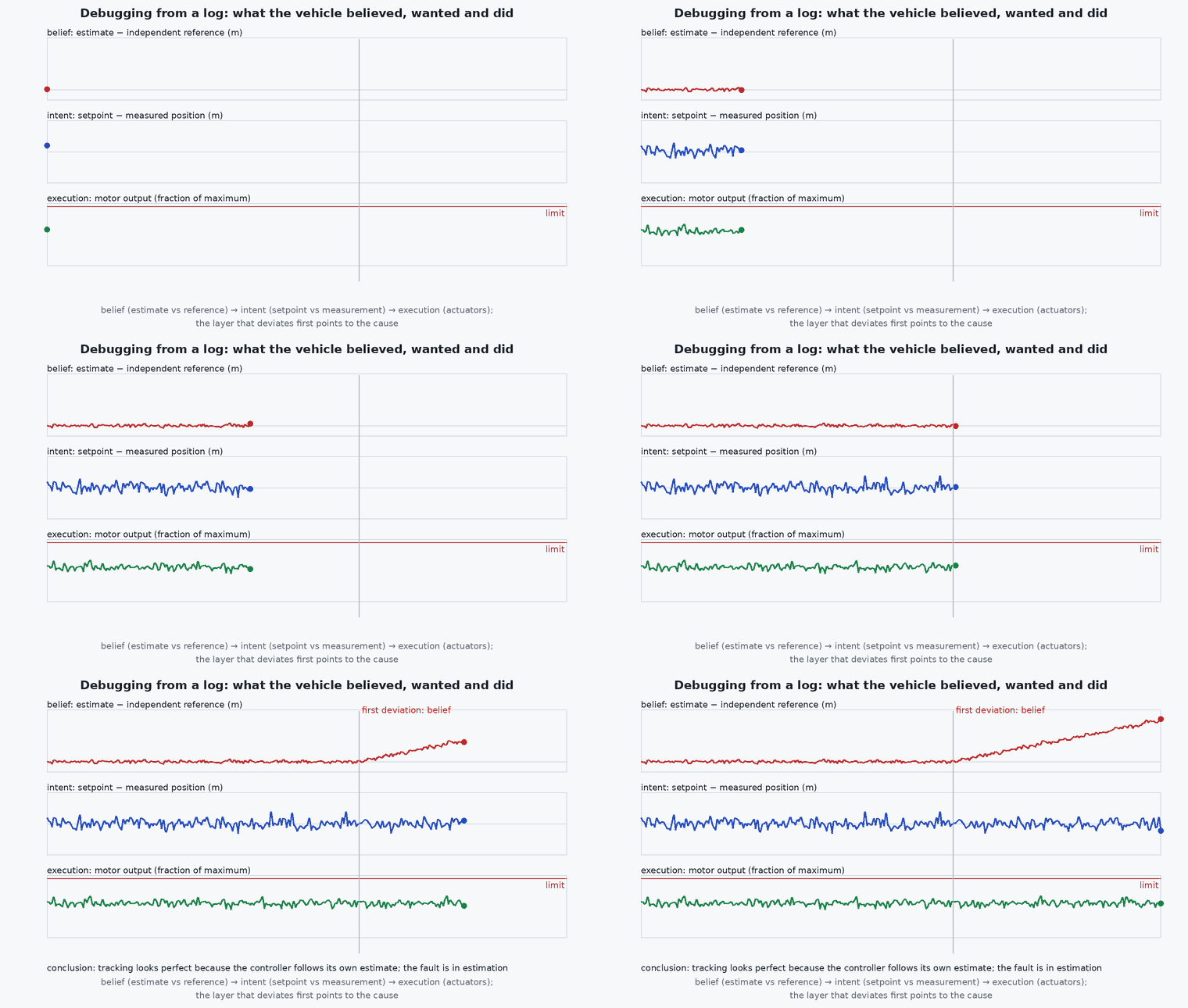
A vehicle can be wrong in three different ways: it can believe something false (estimation), it can want something wrong (setpoint, planner, mode), or it can fail to do what it wanted (controller, actuators, saturation). Each has a typical plot. Beliefs: the estimator’s position against an independent source, innovation test ratios. Intent: the setpoint against time. Execution: setpoint against measured value (tracking), and motor commands against their limits.
Start with the event time, not the whole flight. Zoom to ten seconds before the symptom, plot all three layers together, and ask which one first deviates. Cause precedes effect: the signal that departs first is where to dig.
Mathematical formulation
Three quantities do most of the work. Tracking error and its normalised form, the estimator innovation test ratio (see the EKF2 lesson), and a vibration metric. A common vibration metric is the RMS of the high-pass-filtered accelerometer signal; accelerometer clipping is flagged when samples reach full scale. For a signal sampled at with a high-pass cut-off :
The log time resolution limits what can be seen: a topic logged at 10 Hz cannot show a 20 Hz oscillation (it aliases), so check the logged rate first. Timestamps are microseconds since boot: between messages should be nearly constant; gaps indicate logging dropouts.
- vib_rms
- RMS of the non-gravity component of acceleration .
- logged sample rate; Nyquist limit .
Architecture and data flow
Sensors, estimator, controllers and actuators publish uORB topics → the logger subscribes to a configured set → ring buffer → SD card (or streamed over MAVLink) → .ulg → Flight Review / pyulog / PlotJuggler. For high-rate analysis (vibration spectra, controller internals) enable the corresponding logging profiles; the cost is a larger file and a faster card.
Real-world UAV applications
- Post-flight check of every test flight against acceptance metrics.
- Incident investigation after a crash or failsafe.
- Controller and estimator tuning from recorded data.
- Regression comparison between firmware or parameter versions.
Implementation example
This runs as shown. The analysis functions on a synthetic log (numpy arrays standing in for topics): a logging-dropout detector, a vibration RMS, a tracking-error summary and a first-deviation finder that tells you which layer departed first. For real logs, load the topics with pyulog as in the architecture lesson and pass the arrays to the same functions.
import numpy as np
rng = np.random.default_rng(5)
fs, T = 200, 60.0; t = np.arange(0, T, 1 / fs)

def gaps(ts, nominal_dt, factor=3.0):
    d = np.diff(ts); return ts[:-1][d > factor * nominal_dt]
def vib_rms(acc, fs, fc=5.0):
    a = np.exp(-2 * np.pi * fc / fs); lp = np.zeros_like(acc); lp[0] = acc[0]
    for k in range(1, len(acc)): lp[k] = a * lp[k - 1] + (1 - a) * acc[k]
    return float(np.sqrt(np.mean((acc - lp) ** 2)))
def first_deviation(sig, ref, thresh, ts):
    idx = np.where(np.abs(sig - ref) > thresh)[0]; return float(ts[idx[0]]) if idx.size else None

# synthetic flight: reference position ramps; the estimator develops a bias at t = 30 s; the controller then 'tracks' the wrong position
ref = 0.2 * t; est_err = np.where(t > 30, 0.5 * (t - 30), 0.0); true_pos = ref - est_err              # the controller tracks the estimate, so a bad estimate pulls the true position away
est = true_pos + est_err                                                                                # what the vehicle believes (looks fine against the setpoint)
gps = true_pos + 0.3 * rng.standard_normal(t.size)                                                      # independent reference (e.g. GNSS)
acc = 0.4 * rng.standard_normal(t.size)
ts = t.copy(); ts = np.delete(ts, np.arange(4000, 4080))                                               # a 0.4 s logging dropout

print("dropouts at t =", np.round(gaps(ts, 1 / fs), 2), " vibration rms %.2f m/s^2" % vib_rms(acc, fs))
print("tracking error (est vs setpoint) max %.2f m;  first estimator-vs-GNSS deviation at t = %.1f s" % (np.abs(est - ref).max(), first_deviation(est, gps, 1.5, t)))
assert abs(gaps(ts, 1 / fs)[0] - 19.995) < 0.02
assert 0.2 < vib_rms(acc, fs) < 0.5
assert 31 < first_deviation(est, gps, 1.5, t) < 37 and np.abs(est - ref).max() < 1e-9Common engineering mistakes
Reading only the tracking plot
A good tracking of a wrong estimate looks perfect; compare the estimate with an independent source.
Not logging the topics you need
Configure the logger before the test; a missing topic cannot be recovered.
Analysing the whole flight
Zoom to the event window.
Changing several things between flights
You cannot attribute the result; change one.
Not archiving the log with the parameter file and version
The log is only evidence if the configuration is recorded with it.
Failure modes
| Failure mode | How it shows up | Likely cause |
|---|---|---|
| Log truncated | File ends before landing | Power loss, card error or crash before the buffer flushed |
| Gaps in data | Missing intervals | Logging bandwidth above card throughput |
| Misleading plots | Time axis wrong | Different timestamp bases or aliasing from low logging rate |
| Cannot attribute a failure | Several causes plausible | No independent reference signal logged |
Debugging approach
- Mark the event time and zoom to ±10 s.
- Plot estimate, setpoint and measurement for the affected axis together.
- Check innovation test ratios, vibration and clipping first.
- Check the log text messages (console) for warnings at the event time.
Practical exercises
- Open a Flight Review report for a SITL flight and list the five sections it provides.
- Run the helper functions on a real log and report the dropout count and vibration RMS.
- Write a ten-line incident note: symptom, time, evidence from three layers, hypothesis, next test.
- Add the log of a second flight and compare tracking RMS between parameter sets.
Interview questions
Write an answer in your own words, then reveal the model answer. Nothing is sent anywhere.
Question 1
How do you structure a post-flight log analysis?
Model answer
Mark the event time, then separate estimation (what the vehicle believed), intent (setpoints, mode) and execution (tracking and actuators), look for the first signal to deviate, and test one hypothesis at a time.
Question 2
Why is a good tracking plot not proof that the vehicle behaved well?
Model answer
The controller tracks the estimated state; if the estimate is wrong, tracking can look perfect while the true motion is wrong. Compare against an independent reference.
Question 3
What limits the frequencies you can see in a log?
Model answer
The logging rate: half of it is the Nyquist limit, and higher frequencies alias. Enable high-rate profiles for vibration analysis.
References and further reading
Primary papers, official documentation and standards. Each claim above that is specific to a tool or version points here.