UAV Systems Engineering · Module 3
M3-T2: Gaussian distributions and covariance
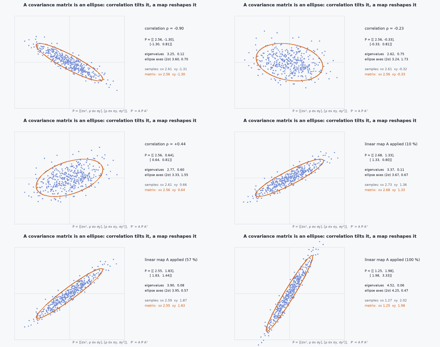
A covariance matrix is an ellipse of belief: its axes say where the vehicle is uncertain and its tilt says which errors move together.
Nearly every UAV estimator assumes Gaussian errors, because the Gaussian is closed under linear maps and conditioning. Reading a covariance matrix as a shape, and propagating it correctly, is the working skill.
Learning objectives
After this lesson, you should be able to:
- Write the multivariate Gaussian and interpret mean and covariance.
- Compute the uncertainty ellipse from the eigen-decomposition and the Mahalanobis distance.
- Propagate covariance through a linear map and through a Jacobian.
- Explain correlation and why dropping off-diagonal terms can make a filter overconfident.
Conceptual explanation
The multivariate Gaussian is fully described by its mean and covariance . The covariance is symmetric positive semi-definite: diagonal entries are variances, off-diagonal entries record how errors move together. Contours of equal probability are ellipsoids: the eigenvectors of are the axes and the square roots of the eigenvalues the semi-axis lengths per standard deviation.
Engineering intuition
In a corridor estimate, along-corridor position may have 2 m uncertainty and across-corridor 0.1 m: a long thin ellipse. The planner needs the thin direction, not the scalar “trace”. Correlation tilts the ellipse: if heading error and cross-track error are positively correlated (a heading error moves the vehicle sideways over time), the ellipse leans, and a measurement that fixes one also improves the other. Discarding the correlation (a diagonal approximation) loses that benefit and often claims more confidence than justified.
Mathematical formulation
Linear map : mean and covariance transform exactly. For a nonlinear map the first-order approximation uses the Jacobian :
Probability inside the k-sigma ellipse of an n-dimensional Gaussian is the chi-square CDF: for , ( = 1: 39%, : 86%, : 99%). Correlation coefficient: . Marginalising a Gaussian drops the rows and columns of the unwanted variables; conditioning gives a Gaussian whose covariance is the Schur complement.
- covariance matrix, symmetric positive semi-definite.
- Jacobian of the nonlinear map at the mean.
- squared Mahalanobis distance (chi-square distributed for a Gaussian).
Architecture and data flow
Filters propagate through (prediction) and shrink it with measurements. Planners should consume the covariance, not just the mean: obstacle margins are inflated along the ellipse’s large axis (lesson M8-T10). When publishing covariance, document the frame and the ordering (position, orientation) of the matrix: ROS covariances are row-major 6×6 in (, , , rotation about , , ).
Real-world UAV applications
- Visualising estimator uncertainty in RViz or a ground station.
- Chance-constrained planning near obstacles.
- Gating measurements by Mahalanobis distance.
- Deciding which sensor to trust in which direction.
Implementation example
This runs as shown: the ellipse of a correlated covariance by eigen-decomposition, Monte Carlo verification of the 2-sigma coverage, linear and Jacobian propagation, and the effect of dropping correlation on a fused estimate.
import numpy as np
rng = np.random.default_rng(1)
S = np.array([[4.0, 1.8], [1.8, 1.0]])                              # strongly correlated 2-D covariance (m^2)
lam, V = np.linalg.eigh(S); print("semi-axes per sigma:", np.round(np.sqrt(lam), 3), "major axis angle (deg):", round(float(np.degrees(np.arctan2(V[1, 1], V[0, 1]))), 1))

x = rng.multivariate_normal([0, 0], S, 200000)
d2 = np.einsum('ij,jk,ik->i', x, np.linalg.inv(S), x)
inside = {k: np.mean(d2 < k * k) for k in (1, 2, 3)}
print("coverage inside k-sigma ellipse:", {k: round(float(v), 3) for k, v in inside.items()})
assert all(abs(inside[k] - (1 - np.exp(-k * k / 2))) < 0.005 for k in (1, 2, 3))

A = np.array([[1.0, 0.5], [0.0, 1.0]]); y = x @ A.T
assert np.allclose(np.cov(y.T), A @ S @ A.T, atol=0.05)             # Sigma_y = A Sigma A^T

r = 10.0; th = np.radians(30); s_r, s_th = 0.1, np.radians(2.0)     # polar to Cartesian: Jacobian propagation
J = np.array([[np.cos(th), -r * np.sin(th)], [np.sin(th), r * np.cos(th)]]); Sy = J @ np.diag([s_r**2, s_th**2]) @ J.T
rr = r + s_r * rng.standard_normal(200000); tt = th + s_th * rng.standard_normal(200000); pts = np.stack([rr * np.cos(tt), rr * np.sin(tt)], axis=1)
assert np.allclose(np.cov(pts.T), Sy, rtol=0.1, atol=0.002)

# dropping correlation: fuse a measurement of the first coordinate; with the full covariance the second coordinate improves too
H = np.array([[1.0, 0.0]]); R = np.array([[0.25]])
def post(P): K = P @ H.T @ np.linalg.inv(H @ P @ H.T + R); return (np.eye(2) - K @ H) @ P
Pf, Pd = post(S), post(np.diag(np.diag(S)))
print("posterior variance of coordinate 2: full", round(float(Pf[1, 1]), 3), "| diagonal approximation", round(float(Pd[1, 1]), 3))
assert Pf[1, 1] < 0.5 * Pd[1, 1]Common engineering mistakes
Dropping off-diagonal terms for convenience
It discards correlation and mis-states uncertainty, often in the wrong direction.
Publishing covariance in the wrong frame or order
ROS orders (, , , roll, pitch, yaw) rotation about axes; mismatches are silent.
Using the trace as the uncertainty
Hides direction: a thin long ellipse and a round one can share a trace.
Propagating through strongly nonlinear maps with a Jacobian
For large uncertainty use sigma points or sampling.
Non-symmetric or non-positive-definite P from rounding
Use the Joseph form and symmetrise.
Failure modes
| Failure mode | How it shows up | Likely cause |
|---|---|---|
| Loss of positive definiteness | Filter produces NaNs | Rounding in covariance update |
| Overconfidence from ignored correlation | NEES high | Diagonal approximation |
| Ellipse in the wrong frame | Planner inflates the wrong direction | Covariance not rotated to the planner frame |
| Linearisation error | Sampled covariance disagrees with | Large uncertainty or strong nonlinearity |
Debugging approach
- Plot ellipses for a few time steps and check their orientation against expectation.
- Compare with a Monte Carlo covariance.
- Check symmetry and eigenvalues of each step.
- Verify that rotating the frame rotates the covariance as .
Practical exercises
- Find the 95% ellipse radius factor for and .
- Compute the covariance in the world frame of a body-frame covariance and a yaw of .
- Show that marginalising removes rows and columns, and that conditioning uses the Schur complement.
- Construct a covariance with correlation 0.9 and plot its ellipse.
Interview questions
Write an answer in your own words, then reveal the model answer. Nothing is sent anywhere.
Question 1
What does the covariance matrix tell you beyond variances?
Model answer
Correlations between errors and the orientation and shape of the uncertainty ellipse, which matter for how a measurement of one quantity improves another.
Question 2
How is covariance propagated through a nonlinear function?
Model answer
To first order as with the Jacobian at the mean; for large uncertainty use sigma points or Monte Carlo.
Question 3
What is Mahalanobis distance used for?
Model answer
Measuring how many standard deviations a point is from the mean in the metric of the covariance: gating and consistency tests.
References and further reading
Primary papers, official documentation and standards. Each claim above that is specific to a tool or version points here.
- . . Barfoot, State Estimation for Robotics, Cambridge University Press, 2017, chapter 2.
- . Bar-Shalom, . . Li, . Kirubarajan, Estimation with Applications to Tracking and Navigation, Wiley, 2001, chapter 1.
- REP 103 (covariance ordering and units conventions in ROS)