UAV Systems Engineering · Module 3
M3-T3: Bayesian estimation
Every filter in this track is the same two steps; they differ only in how the belief is represented.
The Bayes filter is the general recipe for tracking a state from noisy measurements: push the belief through the motion model, then multiply by the measurement likelihood. The Kalman filter, the EKF and the particle filter are different ways of carrying out these two steps.
Learning objectives
After this lesson, you should be able to:
- Write the recursive Bayes filter predict and update equations.
- State the Markov and conditional-independence assumptions behind them.
- Implement a grid (histogram) filter and verify it against a Kalman filter on a linear-Gaussian problem.
- Explain the representation trade-offs: Gaussian, grid and particles.
Conceptual explanation
The Bayes filter maintains the belief . Predict: integrate the previous belief against the motion model . Update: multiply by the measurement likelihood and normalise.
Engineering intuition
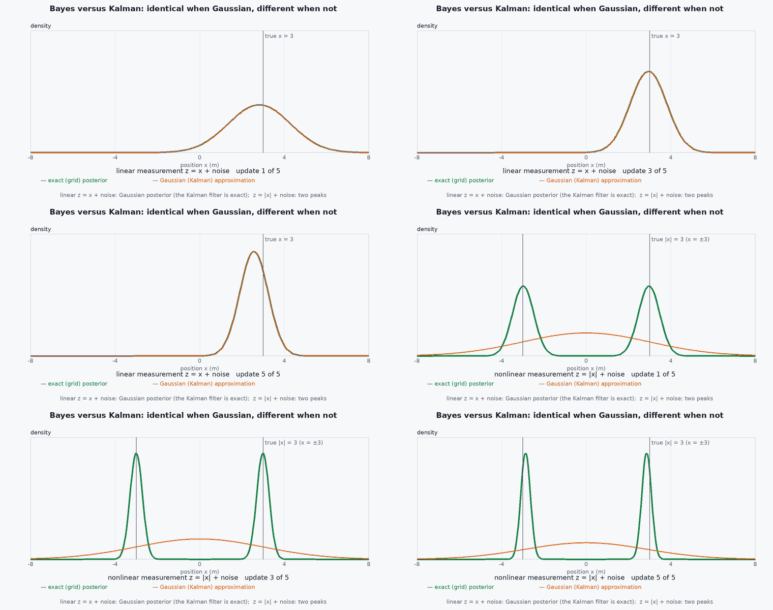
Prediction spreads the belief because the motion is uncertain; the update sharpens it because the measurement is informative. The balance between spreading and sharpening is what “tuning” means. The recursion works because of the Markov assumption: given the current state, the past adds no information about the future, and measurements depend only on the current state. If hidden states are missing from the model (a bias, a delay), the assumption fails and the filter becomes inconsistent: that is why biases are added to the state.
Mathematical formulation
Representations: for linear motion and measurement with Gaussian noise the belief stays Gaussian and the two steps reduce to the Kalman filter equations (lesson M3-T4); linearisation gives the EKF (M3-T5); samples give the particle filter; a grid of cell probabilities gives the histogram filter, exact up to the cell size but exponential in dimension.
- control input (or IMU measurement used as input).
- measurement.
- normaliser.
Architecture and data flow
In a UAV estimator the motion model is the IMU-driven kinematics, the measurements are GNSS, vision and LiDAR, and the belief is a Gaussian over the error state. A grid or particle filter is used for global problems with multimodal beliefs (kidnapped robot, place recognition), where a single Gaussian cannot represent the ambiguity.
Real-world UAV applications
- Understanding what every filter approximates.
- Global localisation against a prior map (Monte Carlo localisation).
- Fusing discrete observations such as landmarks or doors.
- Reasoning about when a Gaussian filter is inadequate (multimodal belief).
Implementation example
This runs as shown: a 1-D grid Bayes filter and a Kalman filter on the same linear-Gaussian problem agree to within the grid resolution.
import numpy as np
rng = np.random.default_rng(2)
q, r, steps, v = 0.3, 0.8, 40, 0.5                          # process std per step, measurement std, steps, commanded velocity per step
xs = np.linspace(-5, 30, 3501); dx = xs[1] - xs[0]           # grid for the histogram filter
gauss = lambda x, m, s: np.exp(-0.5 * ((x - m) / s) ** 2) / (s * np.sqrt(2 * np.pi))

truth = 0.0; bel = gauss(xs, 0.0, 1.0); bel /= bel.sum() * dx          # grid belief
m, P = 0.0, 1.0                                                          # Kalman belief
for k in range(steps):
    truth += v + q * rng.standard_normal(); z = truth + r * rng.standard_normal()
    # predict: convolve with the motion noise (shifted by v) on the grid; Kalman: mean + v, variance + q^2
    kernel = gauss(np.arange(-150, 151) * dx, v, q); kernel /= kernel.sum()
    bel = np.convolve(bel, kernel, mode="same"); bel /= bel.sum() * dx
    m, P = m + v, P + q * q
    # update: multiply by the likelihood; Kalman: scalar gain
    bel = bel * gauss(z, xs, r); bel /= bel.sum() * dx
    K = P / (P + r * r); m, P = m + K * (z - m), (1 - K) * P
mean_grid = (xs * bel).sum() * dx; var_grid = ((xs - mean_grid) ** 2 * bel).sum() * dx
print(f"grid: mean {mean_grid:.3f}, std {np.sqrt(var_grid):.3f} | Kalman: mean {m:.3f}, std {np.sqrt(P):.3f} | truth {truth:.3f}")
assert abs(mean_grid - m) < 0.01 and abs(np.sqrt(var_grid) - np.sqrt(P)) < 0.01 and abs(m - truth) < 4 * np.sqrt(P)Common engineering mistakes
Using a Gaussian filter for a multimodal belief
It averages the modes into a wrong, confident answer; use particles or a grid.
Missing hidden states
A bias not in the state violates the Markov assumption and makes the filter overconfident.
Forgetting to normalise
The belief drifts in scale and the likelihood ratios become meaningless.
Grid too coarse or too large
Resolution error versus exponential cost.
Treating measurement noise as time-varying without modelling
Use the sensor’s covariance per measurement.
Failure modes
| Failure mode | How it shows up | Likely cause |
|---|---|---|
| Particle deprivation | All particles collapse to one wrong cell | Too few particles or too sharp a likelihood |
| Inconsistency | Posterior too narrow | Unmodelled correlations or biases |
| Multimodal ambiguity | Estimate jumps between hypotheses | Gaussian forced on a multimodal belief |
| Numerical underflow | Likelihood product becomes zero | No log-space or normalisation |
Debugging approach
- Compare against the Kalman filter on a linear-Gaussian toy problem.
- Plot the belief over time and check that it narrows and spreads as expected.
- Check that the belief integrates to one.
- Test with a deliberately wrong motion model and see the symptoms.
Practical exercises
- Derive the Kalman gain from the product of two Gaussians.
- Run the grid filter with a bimodal prior and explain why a Kalman filter cannot.
- Add an unknown constant bias to the measurement and see what the filter does.
- Estimate the grid size needed for a 3-D position with 1 cm resolution over 100 m.
Interview questions
Write an answer in your own words, then reveal the model answer. Nothing is sent anywhere.
Question 1
What are the two steps of the Bayes filter?
Model answer
Predict: propagate the belief through the motion model; update: multiply by the measurement likelihood and normalise.
Question 2
What assumptions make the recursion valid?
Model answer
The Markov assumption on the state and conditional independence of measurements given the state.
Question 3
When is a Gaussian belief inadequate?
Model answer
When the true posterior is multimodal, as in global localisation or data association ambiguity; use particles or a grid.
References and further reading
Primary papers, official documentation and standards. Each claim above that is specific to a tool or version points here.
- S. Thrun, W. Burgard, D. Fox, Probabilistic Robotics, MIT Press, 2005, chapter 2
- . . Barfoot, State Estimation for Robotics, Cambridge University Press, 2017, chapter 3.
- A. . Jazwinski, Stochastic Processes and Filtering Theory, Academic Press, 1970.