UAV Systems Engineering · Module 2
M2-T7: Inertial Navigation Systems
An INS is three integrations in a row: it needs no outside signal and gives smooth high-rate pose, but every error it makes is kept and compounded.
The IMU is the one sensor that cannot be jammed, blinded or spoofed. It is also the one that drifts. Understanding exactly how an INS turns raw measurements into pose is the foundation for understanding every fusion filter in this track.
Learning objectives
After this lesson, you should be able to:
- Write the strapdown mechanisation equations for attitude, velocity and position.
- Explain why an accelerometer measures specific force and where gravity enters.
- Identify which IMU errors dominate over which time scales.
- Implement a minimal INS and check it against a known trajectory.
Conceptual explanation
A strapdown INS has sensors rigidly attached to the vehicle. Gyroscopes measure angular rate in the body frame; accelerometers measure specific force in the body frame. The INS integrates the rates into attitude, rotates the specific force into the navigation frame, adds gravity back, and integrates twice to get velocity and position.
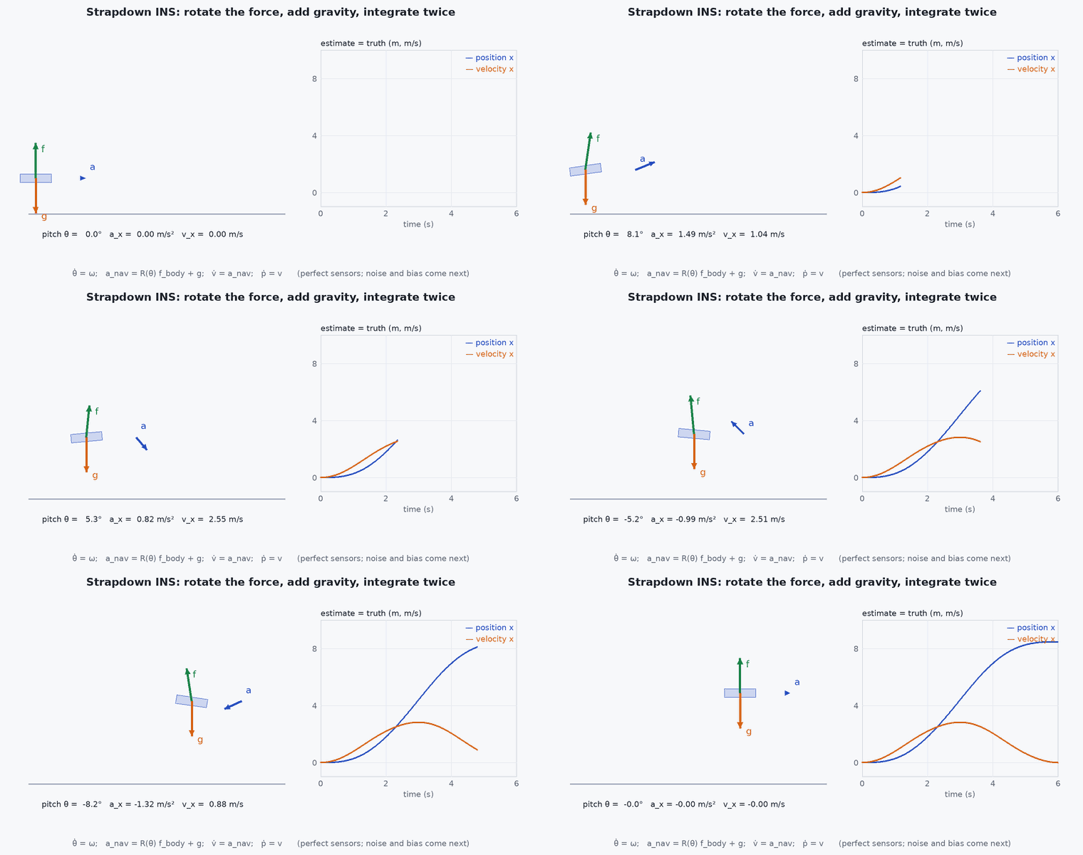
Engineering intuition
Everything an INS knows, it integrated. A tiny constant gyro error becomes an attitude error that grows linearly; that attitude error makes the INS rotate the accelerometer reading the wrong way and project gravity into horizontal acceleration, which is integrated twice. So attitude errors are the nastiest: an attitude error produces a spurious horizontal acceleration of about , and a position error that grows with (lesson M2-T8). This is why every practical system aids the INS with another sensor.
Mathematical formulation
In the navigation frame (here ENU, up), with body-to-navigation rotation , measured angular rate and measured specific force :
- [ω]ₓ
- skew-symmetric matrix of .
- accelerometer output: specific force = a − in the inertial sense, so a stationary level sensor reads +g up.
- gravity vector in the navigation frame.
Over the short flights and small areas typical of UAVs, Earth rotation (15°/h) and curvature can be neglected; for long-range or high-grade navigation they must be included. In discrete time with a sample step , the second-order update is:
Error behaviour
| Error | Cause | Effect on position (small error, constant) |
|---|---|---|
| Accelerometer bias | Sensor offset | ½ |
| Accelerometer noise (velocity random walk) | White noise density | grows as in position |
| Gyro bias | Sensor offset | tilt error gives ≈ ⅙ |
| Initial attitude error | Alignment | ½ horizontally |
Architecture and data flow
IMU (typically 100–1000 Hz) → INS propagation on the autopilot (EKF2 uses the IMU to predict between aiding measurements) → state estimate. Aiding sensors correct it at lower rates. The IMU’s sample timing matters: jitter and missed samples inject errors that look like sensor noise.
Real-world UAV applications
- High-rate attitude and short-term motion estimate used directly by the flight controller.
- Bridging short dropouts of GNSS or vision with dead reckoning.
- Prediction step of every Kalman filter in the track.
- Deskewing LiDAR scans and propagating VIO between camera frames.
Implementation example
This runs as shown: a planar-circle flight is sensed perfectly by a simulated IMU, then integrated. Perfect measurements recover the trajectory; adding a bias or a small attitude error shows the growth.
import numpy as np
dt, T = 0.005, 20.0
g = np.array([0, 0, -9.81])
R_c, w_c = 20.0, 0.25                                  # circle radius (m), angular rate (rad/s)

def truth(t):
    p = np.array([R_c * np.cos(w_c * t), R_c * np.sin(w_c * t), 5.0])
    a = np.array([-R_c * w_c**2 * np.cos(w_c * t), -R_c * w_c**2 * np.sin(w_c * t), 0.0])
    psi = w_c * t + np.pi / 2                          # heading follows the velocity direction
    return p, a, psi

def rotz(a): c, s = np.cos(a), np.sin(a); return np.array([[c, -s, 0], [s, c, 0], [0, 0, 1.0]])

def run(bias=np.zeros(3), tilt_err=0.0):
    p0, a0, psi0 = truth(0.0)
    R = rotz(psi0)
    v = np.array([-R_c * w_c * np.sin(0.0), R_c * w_c * np.cos(0.0), 0.0]); p = p0.copy()
    for k in range(int(T / dt)):
        t = k * dt
        _, a, psi = truth(t)
        Rt = rotz(psi)
        f_body = Rt.T @ (a - g) + bias                 # specific force: a - g, in the body frame, plus bias
        # gyro: exact yaw rate; a constant tilt error rotates the force reading about body x
        Rn = R @ np.array([[1, 0, 0], [0, np.cos(tilt_err), -np.sin(tilt_err)], [0, np.sin(tilt_err), np.cos(tilt_err)]])
        acc = Rn @ f_body + g
        p = p + v * dt + 0.5 * acc * dt**2
        v = v + acc * dt
        R = rotz(psi + w_c * dt)
    return np.linalg.norm(p - truth(T)[0])

e0 = run(); e_bias = run(bias=np.array([0.0, 0.0, 0.0098 * 5])); e_tilt = run(tilt_err=np.radians(0.5))
print(f"perfect {e0:.3f} m | 5 mg z-bias {e_bias:.1f} m | 0.5 deg tilt {e_tilt:.1f} m")
assert e0 < 0.5
assert abs(e_bias - 0.5 * 0.049 * T**2) < 1.0           # 1/2 b t^2 for a vertical bias
assert e_tilt > 5 # a half-degree attitude error is worth metres in 20 sCommon engineering mistakes
Forgetting to add gravity back
The vehicle appears to accelerate upward at 1 : remember the accelerometer reads specific force.
Integrating Euler angles instead of using a rotation or quaternion
Singularities and drift; use exponential map integration with re-normalisation.
Ignoring sample timing
Dropped or jittered IMU samples cause velocity errors that look like noise. Timestamp at acquisition.
Using the INS alone beyond its useful time
Consumer-grade MEMS dead reckoning is useful for seconds, not minutes. Budget the aiding rate accordingly.
Failure modes
| Failure mode | How it shows up | Likely cause |
|---|---|---|
| Gravity compensation error | Constant climb or sink in a hover | Wrong gravity magnitude or an attitude error leaking gravity into horizontal axes |
| Gyro saturation | Attitude jumps after violent manoeuvres | Gyro range exceeded during a flip or crash recovery |
| Vibration rectification | Persistent accelerometer bias that appears only when motors are on | Clipping or aliasing of vibration at the accelerometer |
| Temperature drift | Bias that changes after warm-up | No temperature calibration of the IMU |
Debugging approach
- Sit still and integrate: position should grow as ½ ; fit to the log to estimate the accelerometer bias.
- Hold the vehicle level on a bench and check that the horizontal accelerometer reading is near zero and the vertical near +g.
- Check vibration spectra and clipping flags in the log before trusting any dead reckoning.
- Log IMU timestamps and look for gaps and non-uniform spacing.
Practical exercises
- Derive the position error from a constant accelerometer bias and from a constant gyro bias on a hovering vehicle.
- Run the code with a 0.1 mg bias. How long until position error exceeds 1 m?
- Add Earth’s rotation (15°/h) and see whether it matters over 20 s.
- Replace the exact rotation update with a first-order one and measure the error growth.
Interview questions
Write an answer in your own words, then reveal the model answer. Nothing is sent anywhere.
Question 1
Why does an accelerometer on a table read +1 ?
Model answer
It measures specific force, the non-gravitational force per unit mass. The table’s support force is what it senses; free fall would read zero.
Question 2
Which IMU error is worst for position and why?
Model answer
Attitude error, because it rotates the measured specific force and leaks gravity into horizontal acceleration at about , which becomes position error growing as .
Question 3
Why can’t you just integrate the IMU for position on a drone?
Model answer
Double integration turns even small biases into quadratic position error: a few milli-g bias gives tens of metres within a minute. It needs an aiding sensor.
References and further reading
Primary papers, official documentation and standards. Each claim above that is specific to a tool or version points here.
- . . Groves, Principles of GNSS, Inertial, and Multisensor Integrated Navigation Systems, 2nd ed., Artech House, 2013, chapter 5.
- J. Solà, “Quaternion kinematics for the error-state Kalman filter”, arXiv:1711.02508
- . . Barfoot, State Estimation for Robotics, Cambridge University Press, 2017 (rotations and kinematics).