UAV Systems Engineering · Module 2
M2-T8: Dead reckoning and inertial drift
Position error from inertial navigation grows as t², t^1.5 or t³ depending on the error source; knowing which one dominates tells you how often you must correct.
Every GNSS-denied design starts with one question: how long can the vehicle fly on inertial data alone before the error becomes unacceptable? This lesson turns that question into formulas you can check against a log.
Learning objectives
After this lesson, you should be able to:
- Derive position error growth from a constant accelerometer bias, a gyro bias and white accelerometer noise.
- Estimate the time until inertial position error exceeds a given bound for a given IMU quality.
- Explain why attitude (gyro) errors eventually dominate.
- Fit a bias to a stationary log and predict drift.
Conceptual explanation
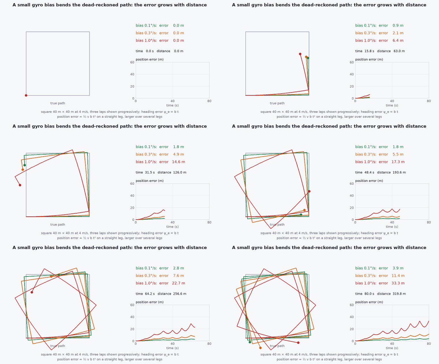
Dead reckoning is estimating position by integrating motion from a known starting point. For an IMU, errors in the measurement are integrated along with the signal. Three sources matter: accelerometer bias (a constant offset), accelerometer noise (random jitter) and gyroscope bias (a constant attitude-rate offset that corrupts the gravity projection).
Engineering intuition
The exponent counts integrations. A bias in acceleration is integrated twice: error ∝ . White noise in acceleration integrates to a random walk in velocity (error ∝ ) and then to position . A gyro bias is integrated once into tilt, which leaks gravity into horizontal acceleration, then twice more: three integrations, . A cheap IMU can therefore look fine for 5 seconds and be metres off at 30.
Mathematical formulation
Accelerometer bias
Accelerometer white noise
For a noise density (m/s²/√Hz), velocity error has standard deviation and position error standard deviation:
Gyro bias
A constant gyro bias gives a tilt error , a spurious horizontal acceleration , and:
- accelerometer bias . 1 mg = .
- gyro bias (rad/s). 1°/s = 0.01745 rad/s.
- accelerometer noise density (m/s²/√Hz): the “velocity random walk” in m/s/√Hz.
- .
The cubic term dominates for above the crossover where ⅙ = ½ , that is . With mg and this is about 86 s. Important: these formulas apply to residual bias after calibration and filtering; consumer MEMS devices can be a lot worse before calibration.
Architecture and data flow
Bias is not constant: it drifts (bias random walk) and depends on temperature. A good estimator therefore estimates the biases online while aiding is available (lesson M3-T7), then dead-reckons with the last estimate during an outage. The residual bias error at the moment aiding is lost sets the drift rate for the whole outage. That is why a short, noisy aiding window just before GNSS loss can be worse than a long clean one earlier.
Real-world UAV applications
- Specifying IMU grade from the maximum allowed outage: how long must the vehicle survive without aiding?
- Choosing when to trigger a failsafe: error bound versus time since last aiding.
- Judging whether a log’s drift is explained by bias or by something else (misalignment, timing).
- Deciding the update rate and covariance inflation in a GNSS-denied estimator.
Implementation example
This runs as shown: it simulates a stationary 1-D accelerometer with bias and noise, fits the bias from the first 10 seconds, and predicts the drift at 60 seconds from the formulas.
import numpy as np
rng = np.random.default_rng(2)
dt, T = 0.01, 60.0
b_a = 0.049                    # 5 mg bias (m/s^2)
N = 0.002                      # noise density, m/s^2/sqrt(Hz)
n = int(T / dt)
acc = b_a + N / np.sqrt(dt) * rng.standard_normal(n)      # stationary: true acceleration is 0

v = np.cumsum(acc) * dt
p = np.cumsum(v) * dt
print(f"position error at 60 s: {p[-1]:.1f} m")

# 1) fit the bias from the first 10 s of stationary data and predict the drift
b_hat = acc[: int(10 / dt)].mean()
pred = 0.5 * b_hat * T**2
print(f"bias estimate {b_hat/9.81*1000:.2f} mg, predicted {pred:.1f} m")
assert abs(pred - p[-1]) / p[-1] < 0.05                    # the bias model explains the drift

# 2) after removing the estimated bias, only noise remains: much smaller growth
acc2 = acc - b_hat
p2 = np.cumsum(np.cumsum(acc2) * dt) * dt
sigma_pred = N * T**1.5 / np.sqrt(3)
print(f"after bias removal: error {abs(p2[-1]):.3f} m, noise-only 1-sigma prediction {sigma_pred:.3f} m")
assert abs(p2[-1]) < 5 * sigma_pred + 0.5 and abs(p2[-1]) < 0.1 * p[-1]Common engineering mistakes
Quoting drift from the noise figure alone
Noise density gives the term; bias gives and usually dominates over minutes. Use both.
Assuming bias is constant over a flight
It drifts with temperature and time (bias instability). Estimate it online and re-estimate often.
Ignoring gravity leakage from attitude error
Even a perfect accelerometer drifts if the attitude is wrong by a fraction of a degree.
Comparing datasheet numbers without units
mg versus , versus rad/s, and per √Hz versus per hour are the usual traps.
Failure modes
| Failure mode | How it shows up | Likely cause |
|---|---|---|
| Quadratic drift on a vertical-only axis | Altitude slowly climbs or sinks during dead reckoning | Accelerometer z-bias not removed |
| Cubic growth after a quiet start | Fine for 20 s and then rapidly worse | Gyro bias residual leaking gravity into horizontal channels |
| Covariance too small during an outage | Estimator overconfident while drifting | Process noise does not include bias random walk |
| Temperature-induced bias step | Sudden drift after power-up warm-up | No thermal calibration, or heating from the companion computer |
Debugging approach
- Place the vehicle still, log for a minute and compute the mean and Allan deviation of each axis.
- Fit ½ to the integrated position of the stationary data to recover .
- Check the temperature trace against bias in a warm-up test.
- Verify that the estimator’s covariance during a simulated outage grows at least as fast as the true error.
Practical exercises
- How long until position error exceeds 10 m for a 2 mg bias? And 1 m?
- Find the crossover time at which gyro-bias drift overtakes accelerometer-bias drift for mg and .
- If you must survive a 30 s GNSS outage within 5 m, what accelerometer bias residual is acceptable?
- Use the Sensor Fusion Simulator to reproduce the growth with fusion disabled.
Interview questions
Write an answer in your own words, then reveal the model answer. Nothing is sent anywhere.
Question 1
What growth law does a constant accelerometer bias produce in position?
Model answer
Quadratic: = ½ , because the bias is integrated twice.
Question 2
Why does a small gyro bias eventually dominate?
Model answer
It causes tilt that grows linearly, which leaks gravity into horizontal acceleration and is integrated twice more, giving ≈ ⅙ , a cubic term.
Question 3
How do you reduce inertial drift during a GNSS outage?
Model answer
Estimate and remove biases while aiding is available, use a better IMU, add other aiding sensors (vision, LiDAR, airspeed), and reduce the outage duration by detecting and responding sooner.
References and further reading
Primary papers, official documentation and standards. Each claim above that is specific to a tool or version points here.
- . . Groves, Principles of GNSS, Inertial, and Multisensor Integrated Navigation Systems, 2nd ed., Artech House, 2013.
- IEEE Std 952-1997, Guide for the specification of inertial sensors (Allan variance method; check current revision)
- . . Barfoot, State Estimation for Robotics, Cambridge University Press, 2017.