UAV Systems Engineering · Module 2
M2-T16: Multi-sensor GNSS-denied navigation architectures
No single sensor survives every environment: design for diverse aiding sources, honest uncertainty and a manager that knows what to do when they disagree.
Each aiding sensor has a failure mode the others do not: GNSS is blocked or spoofed, cameras need light and texture, LiDAR needs geometry. A robust GNSS-denied UAV is therefore an architecture, not an algorithm: diversity, monitoring and a policy.
Learning objectives
After this lesson, you should be able to:
- Explain the complementary failure modes of GNSS, vision, LiDAR and inertial sensing.
- Draw a layered architecture with an IMU-driven core, monitored aiding sources and a navigation manager.
- Define navigation confidence levels and the modes they trigger.
- Choose between loosely and tightly coupled integration for a given design.
Conceptual explanation
A layered GNSS-denied architecture has four parts: (1) an IMU-driven core estimator that always runs and provides continuous, smooth state; (2) aiding sources (GNSS, visual-inertial odometry, LiDAR-inertial odometry) that correct its drift; (3) monitors attached to each source, which publish health and covariance; (4) a navigation manager that turns monitor outputs into a confidence level and a mode.
| Sensor | Strength | Fails when | Failure signature |
|---|---|---|---|
| IMU | Always available, high rate | Never blocked; always drifts | Quadratic position growth |
| GNSS | Global, no drift | Blocked, jammed, spoofed | Fix lost or confident but wrong |
| Camera (VIO) | Rich, cheap, precise relative motion | Dark, textureless, blurred, dynamic | Few features, low inliers |
| LiDAR (LIO) | Direct geometry, independent of light | Degenerate geometry, dust or rain, vibration | Registration residual high, one direction unconstrained |
| Radar | Works in dust, fog, dark; Doppler velocity | Low resolution, multipath | Sparse returns |
Engineering intuition
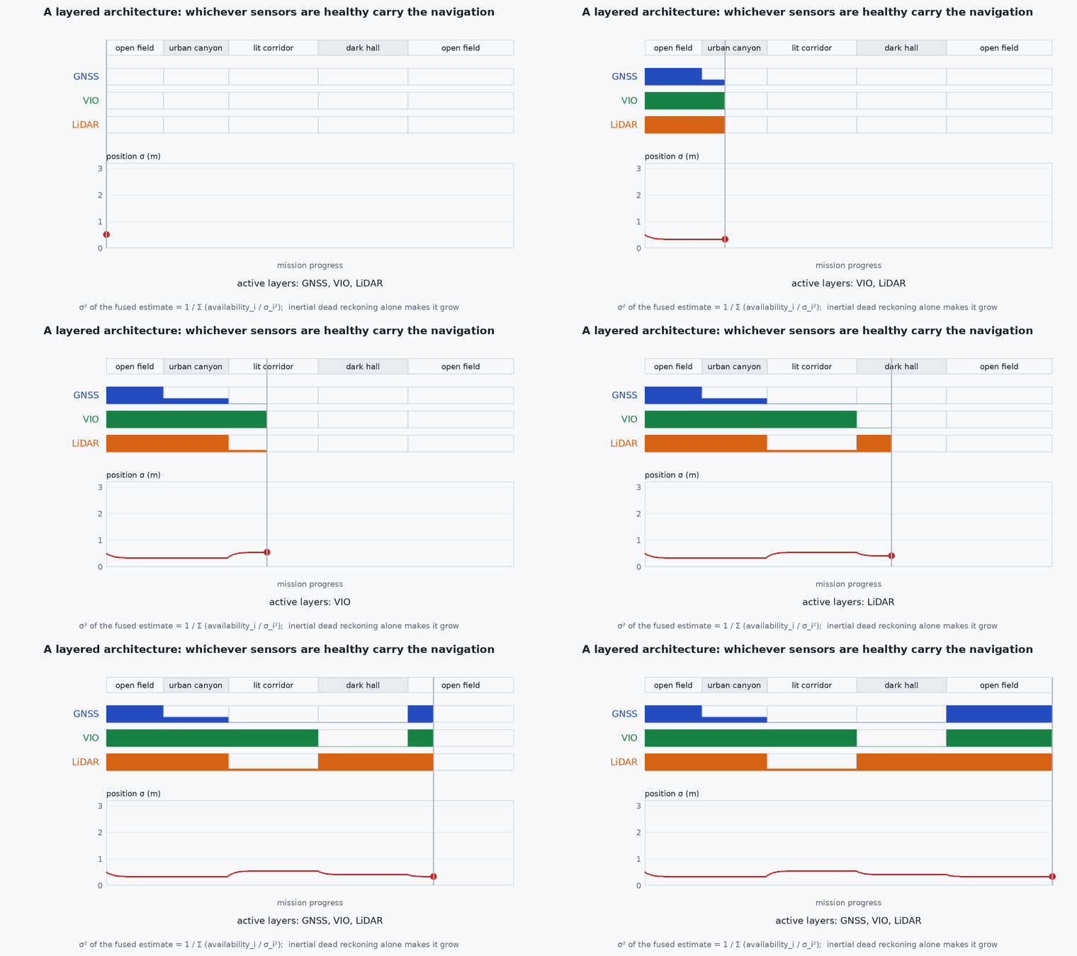
Choose the aiding sources so that a condition that kills one rarely kills the other: a dark corridor defeats vision but gives LiDAR strong structure on both walls and floor; a long featureless corridor can defeat LiDAR geometry but a lit, textured wall helps vision. Diversity beats redundancy of the same type. And what matters as much as the sensors is knowing when each is lying: the manager must see health and covariance, and the estimator must inflate uncertainty honestly when a source degrades, or the confidence metric is meaningless.
Mathematical formulation
Loose versus tight coupling
Loosely coupled: each odometry subsystem produces its own pose (and covariance); the core filter fuses those poses as measurements. Simple and modular, but the subsystem’s internal uncertainty is approximated by a single covariance and correlations are lost. Tightly coupled: the filter or optimiser processes raw features or scan residuals together with IMU, so it can still extract information when too few features exist for a standalone pose.
Confidence
One workable definition combines the estimator’s covariance and the source health:
- one-sigma position uncertainty from the estimator’s covariance (m).
- ,
- thresholds derived from the mission requirement (for example allowed error against the smallest clearance) and verified in test.
Thresholds are requirements, not defaults: derive them from the smallest margin the mission must respect (module 8, lesson M8-T1).
Mode logic
| Confidence | Mode | Typical response |
|---|---|---|
| GREEN | Nominal | Full mission |
| AMBER | Degraded (GNSS-denied, odometry only) | Reduce speed, increase clearances, no new mission legs into unmapped areas |
| RED | Dead reckoning | Hold or return along a known path while the clock runs |
| RED for too long | Failsafe | Controlled stop, land or return |
Architecture and data flow
Monitors publish a small health record per source: timestamp, validity, covariance (or inflation factor), and specific indicators (feature count, inlier ratio, registration residual, satellite count, NIS). The estimator publishes state and covariance. The manager consumes both and publishes mode and confidence to the planner and mission layer; the planner uses them to bound speed and choose conservative paths. This record format is an interface worth writing in the ICD (lesson M7-T17).
Real-world UAV applications
- Warehouse, tunnel and under-canopy inspection where GNSS is unavailable.
- Urban delivery where GNSS degrades between buildings.
- Search and rescue in collapsed structures with dust and darkness (LiDAR and radar over vision).
- Defence and critical infrastructure where jamming and spoofing are expected.
Implementation example
This runs as shown: a small, testable navigation manager. Feed it monitor outputs and it returns the confidence level and mode, with a failsafe timer.
from dataclasses import dataclass

@dataclass
class Health:
    gnss_ok: bool
    vio_ok: bool
    lio_ok: bool
    sigma_pos: float        # estimator 1-sigma position uncertainty (m)

class NavManager:
    def __init__(self, s_green=3.0, s_amber=10.0, red_timeout=8.0):
        self.s_green, self.s_amber, self.red_timeout = s_green, s_amber, red_timeout
        self.red_since = None; self.failsafe = False

    def update(self, t, h: Health):
        odo = h.vio_ok or h.lio_ok
        if h.sigma_pos < self.s_green and h.gnss_ok and odo:
            conf = "GREEN"                      # GNSS and odometry agree and the estimate is tight
        elif h.sigma_pos < self.s_amber and (odo or h.gnss_ok):
            conf = "AMBER"                      # one kind of aiding left, uncertainty bounded
        else:
            conf = "RED"
        if conf == "RED":
            self.red_since = t if self.red_since is None else self.red_since
            if t - self.red_since > self.red_timeout: self.failsafe = True
        else:
            self.red_since = None
        mode = "FAILSAFE" if self.failsafe else {"GREEN": "NOMINAL", "AMBER": "DEGRADED", "RED": "DEAD_RECKONING"}[conf]
        return conf, mode

m = NavManager()
assert m.update(0.0, Health(True, True, False, 0.4)) == ("GREEN", "NOMINAL")
assert m.update(1.0, Health(False, True, False, 0.8)) == ("AMBER", "DEGRADED")        # GNSS lost, vision aids
assert m.update(2.0, Health(False, False, False, 2.5))[0] == "RED"                    # nothing aiding
assert m.update(9.0, Health(False, False, False, 6.0)) == ("RED", "DEAD_RECKONING")   # 7 s: still within the timeout
assert m.update(11.0, Health(False, False, False, 9.0)) == ("RED", "FAILSAFE")        # 9 s of RED: failsafe latches
print("navigation manager behaves as specified")Common engineering mistakes
Two sensors with the same failure mode
Two cameras both fail in darkness. Choose diversity: vision plus LiDAR or radar.
Monitors that report only valid or invalid
Report covariance and indicators; the manager needs graded information.
A failsafe with no tested trigger
If the RED timer has never fired in test, you do not know what the vehicle does when it does.
Letting the estimator be overconfident
Honest covariance is what makes the confidence level meaningful (lessons M3-T12 to M3-T15).
Binding the mission to GNSS-only geofences
A geofence evaluated on a drifted estimate is not a geofence.
Failure modes
| Failure mode | How it shows up | Likely cause |
|---|---|---|
| Common-mode failure | All aiding sources degrade together | Darkness plus dust, or a long featureless tunnel defeating both vision and LiDAR geometry |
| Silent drift | Estimate wrong while confidence stays GREEN | Overconfident covariance, monitors missing a degradation |
| Mode chatter | Rapid toggling between modes | No hysteresis around thresholds |
| Late failsafe | Error exceeds clearance before RED timer expires | Timeout chosen without relating drift rate to mission margins |
Debugging approach
- Replay logged data with each sensor removed in turn and watch confidence and mode; any case that stays GREEN is a gap.
- Compare reported to actual error against an external reference: the error should rarely exceed .
- Check hysteresis by sweeping a monitored value up and down across a threshold.
- Review the log for the latency from fault onset to mode change.
Practical exercises
- Choose sensors for a mine-shaft inspection UAV and justify the diversity.
- Add hysteresis to the manager above so that it returns to GREEN only after 3 s of good health.
- Derive a RED timeout from a drift rate of 0.2 m/s and a 2 m clearance margin.
- In the GNSS-Denied Failure Simulator, find a fault pair that defeats the architecture without triggering the failsafe in time.
Interview questions
Write an answer in your own words, then reveal the model answer. Nothing is sent anywhere.
Question 1
Why prefer sensor diversity over redundancy?
Model answer
Redundant identical sensors fail together in the same conditions (common-mode failure). Diverse sensors have different failure modes, so one usually survives.
Question 2
What must a navigation monitor publish besides position?
Model answer
Validity and uncertainty: covariance or inflation, plus health indicators such as feature count, inlier ratio, registration residual and innovation statistics, so a manager can grade confidence.
Question 3
What is the difference between loosely and tightly coupled fusion?
Model answer
Loose fusion treats a subsystem’s pose as a measurement; tight fusion uses raw features or residuals in the filter, preserving correlations and working with fewer features, at higher complexity.
References and further reading
Primary papers, official documentation and standards. Each claim above that is specific to a tool or version points here.
- . . Groves, Principles of GNSS, Inertial, and Multisensor Integrated Navigation Systems, 2nd ed., Artech House, 2013 (integration architectures and integrity).
- T. Qin et al., “A general optimization-based framework for local odometry estimation with multiple sensors”, arXiv:1901.03638 (the VINS-Fusion local odometry framework)
- PX4: external position estimation