UAV Systems Engineering · Module 2
M2-T15: Radar-aided navigation
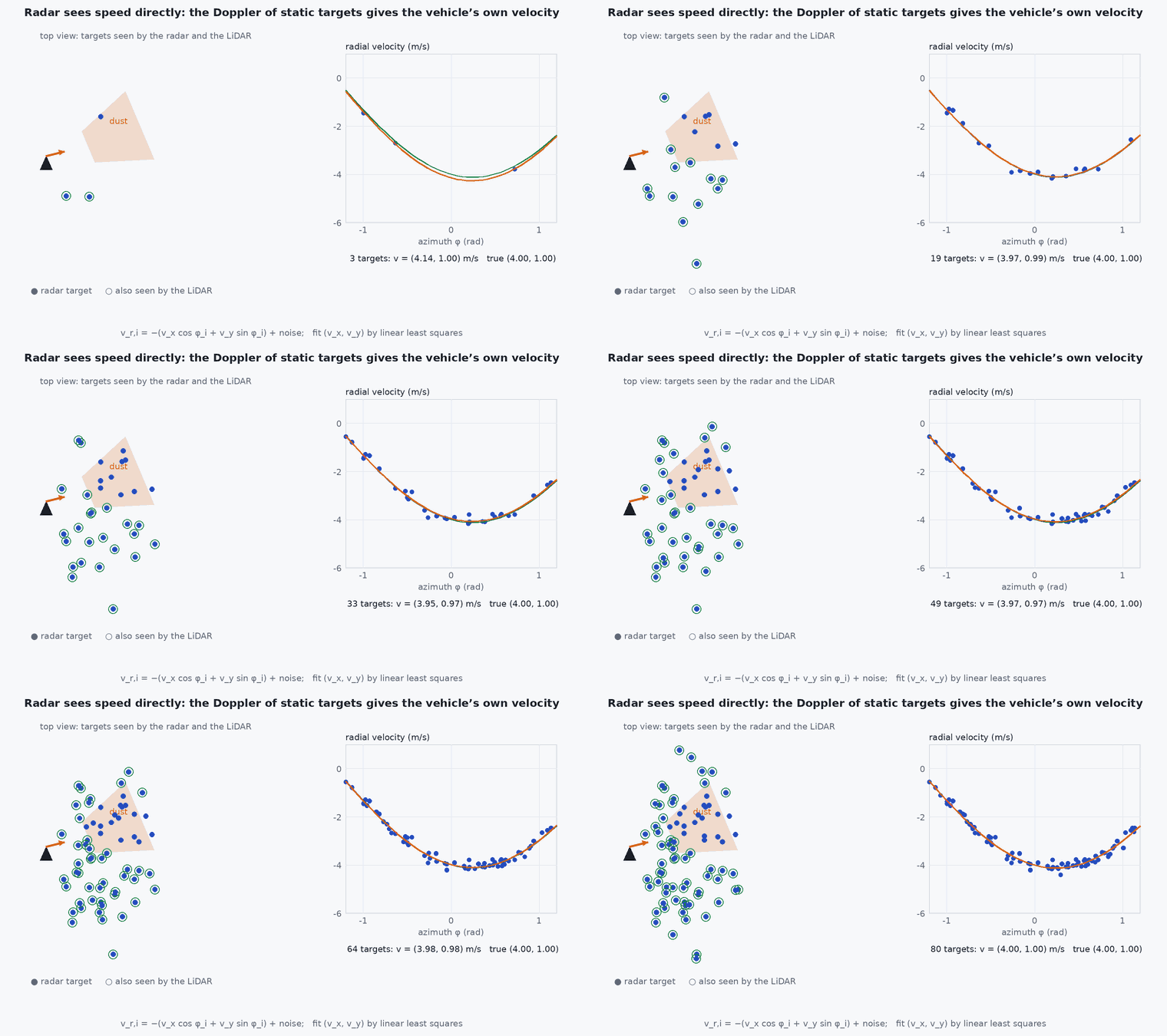
Radar measures velocity directly, in the dark and through dust: each stationary target tells you the vehicle’s speed along the line of sight.
Where cameras and LiDAR struggle (smoke, dust, fog, rain, darkness), radar keeps working. It is lower resolution, but its Doppler measurement turns the whole environment into a velocity sensor. This lesson derives the ego-motion estimate and shows its robustness to moving targets.
Learning objectives
After this lesson, you should be able to:
- Explain what a radar measures (range, azimuth, elevation, radial velocity) and its limits.
- Derive ego velocity from the radial velocities of stationary targets.
- Reject moving targets with RANSAC.
- State where radar helps and where it does not.
Conceptual explanation
A radar emits electromagnetic waves and measures reflections. Modern compact (FMCW) radars give each detection a range, azimuth (and for 4-D radars, elevation) and a radial (Doppler) velocity. Wavelengths of millimetres pass through dust, smoke, fog and rain and do not depend on light. The price is coarse angular resolution, sparse and noisy point clouds, ghost targets from multipath, and specular reflection.
Engineering intuition
If you drive past a stationary sign, its Doppler shift says how fast you approach it along the line of sight. Every stationary object around you does the same, each along its own direction. A handful of detections in different directions pins down the full velocity vector. Moving objects (people, vehicles) violate the assumption, which is why a robust fit is used. Because the Doppler is a direct velocity measurement, drift is much lower than integrating accelerations, though position still accumulates error by integrating velocity.
Mathematical formulation
A stationary target at unit direction (sensor frame) produces radial velocity for sensor velocity . Stacking detections:
The conditioning of depends on the spread of directions: detections only straight ahead cannot give the lateral velocity (the same geometric degeneracy as for LiDAR). RANSAC: sample three detections (or two for planar motion), solve, count inliers with < threshold, keep the best, refit. For rotation, a second antenna or gyro is used; the lever-arm velocity ω × rsensor must be removed.
- radial velocity of detection (positive when moving away, by convention: check your sensor).
- unit vector from the sensor to the target.
- measurement noise; includes moving targets as outliers.
Architecture and data flow
Radar point cloud with Doppler → ego-velocity estimator with RANSAC → velocity with covariance (from the residuals and geometry) → estimator as a velocity measurement alongside IMU (lesson M3-T10 style fusion), and optionally as a scan-registration source with radar-specific methods (research level). Calibrate the radar-to-IMU extrinsics and check the sign convention of the radial velocity.
Real-world UAV applications
- Flight in smoke, dust and fog where optical sensors fail.
- Velocity aiding with no dependence on texture or geometry.
- Altitude and terrain-following with radar altimeters.
- Diverse redundancy to vision and LiDAR (lesson M2-T16).
Implementation example
This runs as shown: radar detections of stationary points plus moving targets; a RANSAC ego-velocity estimator recovers the vehicle velocity within a few centimetres per second where plain least squares is biased by the movers.
import numpy as np
rng = np.random.default_rng(6)
v_true = np.array([3.0, -0.8, 0.5])                                  # vehicle velocity in the sensor frame (m/s)

N = 120
dirs = rng.standard_normal((N, 3)); dirs[:, 0] = np.abs(dirs[:, 0]) + 0.3; dirs /= np.linalg.norm(dirs, axis=1, keepdims=True)   # detections in a forward-looking cone
vr = -dirs @ v_true + 0.05 * rng.standard_normal(N)                  # radial velocity of stationary targets
movers = rng.choice(N, 25, replace=False)                            # 25 detections are on moving objects
vr[movers] += rng.uniform(-6, 6, len(movers))

def lsq(U, y): return np.linalg.lstsq(-U, y, rcond=None)[0]
def ransac_ego(U, y, iters=200, thresh=0.25):
    best, best_in = None, None
    for _ in range(iters):
        idx = rng.choice(len(U), 3, replace=False); v = lsq(U[idx], y[idx])
        inl = np.abs(y + U @ v) < thresh
        if best_in is None or inl.sum() > best_in.sum(): best, best_in = v, inl
    return lsq(U[best_in], y[best_in]), best_in

v_plain = lsq(dirs, vr); v_rob, inl = ransac_ego(dirs, vr)
print(f"plain least squares error {np.linalg.norm(v_plain - v_true):.2f} m/s, RANSAC error {np.linalg.norm(v_rob - v_true):.3f} m/s, inliers {inl.sum()} of {N}")
assert np.linalg.norm(v_rob - v_true) < 0.05 and np.linalg.norm(v_plain - v_true) > 3 * np.linalg.norm(v_rob - v_true)
assert not np.any(inl[movers[np.abs(vr[movers] + dirs[movers] @ v_true) > 1.0]]) # the clearly moving targets were rejectedCommon engineering mistakes
Assuming all detections are stationary
Movers bias a plain fit; use RANSAC or a Doppler-based classifier.
Wrong sign convention of radial velocity
The estimated velocity is mirrored: check with a known motion.
Ignoring lever arm and rotation
Angular rate adds to the sensor velocity.
Expecting LiDAR-like point density
Radar is sparse and noisy; design the estimator for that.
Ghost targets
Multipath produces detections at wrong positions; use consistency.
Failure modes
| Failure mode | How it shows up | Likely cause |
|---|---|---|
| Lateral velocity unobservable | Wrong sideways velocity | All detections near the boresight |
| Moving crowd | Estimate pulled | Many movers, RANSAC threshold too loose |
| Metallic reflections | Ghost detections near walls | Multipath |
| Interference | Noisy detections | Other radars on the same band |
Debugging approach
- Plot radial velocity against · of the estimated velocity: stationary targets should lie on a line.
- Compare against another velocity source.
- Check the sign convention with a straight-line drive.
- Examine detection density against the field of view.
Practical exercises
- Show that detections in only one direction cannot determine lateral velocity.
- Add rotation: include and estimate both.
- Choose a RANSAC threshold for a 0.1 m/s noise and justify it.
- Describe how radar would complement vision and LiDAR in a smoke-filled tunnel.
Interview questions
Write an answer in your own words, then reveal the model answer. Nothing is sent anywhere.
Question 1
What does a radar give that vision and LiDAR do not?
Model answer
Direct radial velocity (Doppler) and operation in dust, smoke, fog and darkness.
Question 2
How is ego velocity estimated from radar?
Model answer
For stationary targets the radial velocity is minus the line-of-sight direction dotted with the vehicle velocity; a robust least-squares fit over many detections gives the velocity.
Question 3
What are radar’s weaknesses for navigation?
Model answer
Low angular resolution, sparse and noisy detections, multipath ghosts and specular effects.
References and further reading
Primary papers, official documentation and standards. Each claim above that is specific to a tool or version points here.
- S. H. Cen, P. Newman, “Precise ego-motion estimation with millimeter-wave radar under diverse and challenging conditions”, ICRA 2018
- Texas Instruments: FMCW radar fundamentals (application note)
- . A. Richards, Fundamentals of Radar Signal Processing, 2nd ed., McGraw-Hill, 2014.