UAV Systems Engineering · Module 5
M5-T2: Quadrotor dynamic modelling
A model is only as good as its parameters: measure mass, inertia, thrust curve and motor lag, then check the model against a log.
The equations of lesson M1-T5 need numbers. This lesson shows how to obtain them from bench measurements and flight data, and how to choose an integration step so that the simulator itself is not the source of error.
Learning objectives
After this lesson, you should be able to:
- List the parameters of a quadrotor model and how each is measured.
- Estimate inertia from a pendulum test and the motor time constant from a step response.
- Choose an integration scheme and step size for the stiff motor dynamics.
- Validate the model against flight data by comparing step responses.
Conceptual explanation
The model needs: mass , centre of mass and inertia , arm geometry, the propeller thrust and drag-torque as functions of rotor speed ( = T Ω², = Q Ω² as the standard approximation), the motor and ESC time constant and limits, aerodynamic drag, and sensor models. Parameters from CAD are a starting point; measured values replace them.
Engineering intuition
Not all parameters matter equally for the controller you are tuning: the attitude loop is dominated by inertia and the motor lag; altitude hold by thrust-to-weight and the thrust curve; position hold by drag. Measure those first. The validation step is the honest one: command a small attitude step in flight, compare it with the same step in the model; mismatch in rise time points to inertia or motor lag, mismatch in overshoot to damping or delay.
Mathematical formulation
Thrust and drag torque from rotor speed, first-order motor dynamics, and the discretisation:
Inertia about a horizontal axis from a pendulum test with period (small oscillations), mass , suspension height from the centre of mass and the suspension’s own inertia negligible:
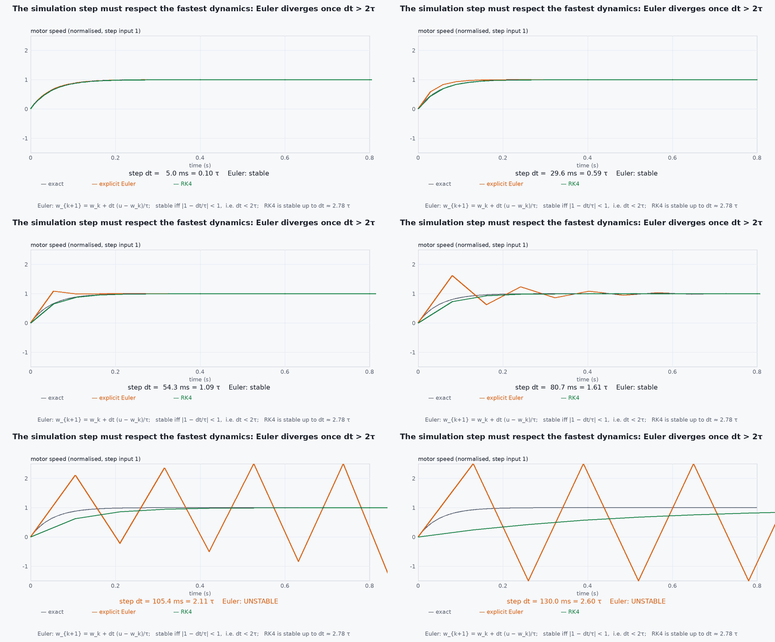
Motor time constant from a step response: the time to reach 63.2% of the final value. Integration: the fastest dynamics set the step; with an explicit Euler step above about is unstable, while the exact exponential update is stable for any ; choose for accuracy of the rest.
Thrust, weight and the sign of gravity
The rotor model feeds the translational equation of lesson M1-T5. With up, the total thrust is along the body axis and the equation is
The weight is not negative: its size is positive (14.7 for a 1.5 kg vehicle). The minus sign is its direction. points up and gravity pulls down, so the weight vector is . On the vertical axis, level thrust gives +T and the weight −mg, so . In a simulator this is one line, a = R @ [0, 0, T] / m - [0, 0, g]. In a z-down frame (NED) points down, the weight is +mg and thrust is − ; the physics is the same, so pick one convention for the whole simulator and convert at the boundary.
Hover is the case : the four rotors must together produce . With equal rotor speeds this fixes the hover speed, and it is the number to check first when a simulated or real vehicle climbs or sinks at zero command:
- ,
- thrust and torque coefficients (N/(rad/s), ·m/(rad/s)).
- motor-ESC time constant.
- ,
- pendulum period and distance from pivot to the centre of mass.
Architecture and data flow
Parameter file (YAML) shared by simulator, controller design scripts and planner; versioned with the airframe (lesson M7-T19). Gazebo vehicle models used with PX4 SITL have their own parameter sets: keep them aligned with your measured values if you want SITL to predict your flight.
Real-world UAV applications
- Tuning in simulation before the first flight.
- Checking that a payload change leaves the controller stable.
- Model-based estimators and MPC.
- Detecting a damaged motor from a changed time constant.
Implementation example
This runs as shown: inertia from a simulated pendulum test, motor time constant fitted from a noisy step response, and the stability of explicit Euler versus the exact update.
import numpy as np
rng = np.random.default_rng(0)
g = 9.81

# 1) inertia from a pendulum test: the airframe hangs on a pivot 0.12 m above its centre of mass
m, d, J_true = 1.5, 0.12, 0.020
P_true = 2 * np.pi * np.sqrt((J_true + m * d * d) / (m * g * d))                   # the period the experiment would give
P_meas = P_true * (1 + 0.005 * rng.standard_normal())                              # 0.5 % timing error
J_est = m * g * d * P_meas ** 2 / (4 * np.pi ** 2) - m * d * d
print(f"inertia: true {J_true:.4f}, estimated {J_est:.4f} kg m^2")
assert abs(J_est - J_true) / J_true < 0.10

# 2) motor time constant from a noisy step response (command 0 -> 1000 rad/s at t = 0)
tau_true, dt = 0.030, 0.002; t = np.arange(0, 0.3, dt); omega = 1000 * (1 - np.exp(-t / tau_true)) + 8 * rng.standard_normal(len(t))
A = np.stack([t, np.ones_like(t)], axis=1); y = np.log(np.clip(1 - omega / 1000, 1e-3, None)); m_ = t < 0.09                 # fit the early part of the decay
slope = np.linalg.lstsq(A[m_], y[m_], rcond=None)[0][0]; tau_est = -1 / slope
print(f"motor time constant: true {tau_true * 1000:.0f} ms, fitted {tau_est * 1000:.1f} ms")
assert abs(tau_est - tau_true) / tau_true < 0.2

# 3) explicit Euler versus the exact update for the first-order motor
def euler(dt, tau, n=200):
    w = 0.0
    for _ in range(n): w += (1000 - w) / tau * dt
    return w
def exact(dt, tau, n=200):
    w = 0.0
    for _ in range(n): w = 1000 + (w - 1000) * np.exp(-dt / tau)
    return w
assert abs(euler(0.001, 0.03, 300) - 1000) < 1.0 and abs(euler(0.07, 0.03) - 1000) > 1e6          # explicit Euler diverges when dt > 2 tau
assert abs(exact(0.07, 0.03) - 1000) < 1e-6 # the exact update is stable for any stepCommon engineering mistakes
Taking inertia from CAD without the wiring and battery
Measured inertia differs by tens of percent.
Using a quasi-static thrust curve for fast manoeuvres
Motor lag matters: include it.
Explicit Euler with a large step on stiff dynamics
Instability or numerical damping; use the exact exponential or a smaller step.
Identifying on one battery voltage
Thrust and lag change with voltage.
Skipping validation
The model may match the bench and not the flight.
Failure modes
| Failure mode | How it shows up | Likely cause |
|---|---|---|
| Simulation stable, vehicle oscillates | Real vehicle rings at the attitude loop bandwidth | Motor lag or delay not modelled |
| Hover thrust mismatch | Simulated hover throttle differs from the real one | Thrust curve wrong |
| Yaw too slow or too fast | Yaw response differs | Drag torque coefficient wrong |
| Numerical blow-up | NaN in simulation | Integration step too large |
Debugging approach
- Compare step responses of roll rate between model and log.
- Check hover throttle in the log against the model.
- Run the simulation at half the step and see whether results change.
- Plot ESC command and measured rpm to estimate .
Practical exercises
- Compute the inertia error if the centre-of-mass offset is mis-measured by 5 mm.
- Design a step test for the yaw axis and the fit to extract .
- Show that the exact update equals the analytic step response.
- Measure your own vehicle’s hover throttle and compare with the model.
Interview questions
Write an answer in your own words, then reveal the model answer. Nothing is sent anywhere.
Question 1
How do you measure a quadrotor’s inertia?
Model answer
With a pendulum or bifilar test: measure the oscillation period and use the pendulum formula with the pivot geometry, subtracting the parallel-axis term.
Question 2
Why does the motor time constant matter?
Model answer
It adds phase lag inside the attitude loop and limits achievable bandwidth; models without it predict better stability than the vehicle has.
Question 3
How would you validate a model?
Model answer
Apply the same small command to the vehicle in flight and to the model and compare the responses (rise time, overshoot, settling).
References and further reading
Primary papers, official documentation and standards. Each claim above that is specific to a tool or version points here.
- R. Mahony, V. Kumar, P. Corke, IEEE RAM 2012
- PX4: simulation (vehicle model parameters)
- . . Beard, . . McLain, Small Unmanned Aircraft, Princeton University Press, 2012, appendix on parameter identification.