UAV Systems Engineering · Module 1
M1-T5: Six-degree-of-freedom UAV dynamics
Twelve numbers describe where a rigid quadrotor is and how it is moving; two vector equations say how they change.
A quadrotor is a rigid body pushed by four thrust forces. That single fact gives you the model every controller, estimator and simulator in this track is built on. This lesson writes it down, explains each term, and integrates it.
Learning objectives
After this lesson, you should be able to:
- List the 12 states of a rigid-body UAV and their frames.
- Write the translational and rotational equations of motion with thrust and torque as inputs.
- Explain why a quadrotor is underactuated and how tilt produces horizontal acceleration.
- Integrate the model numerically and verify hover and a free fall.
Conceptual explanation
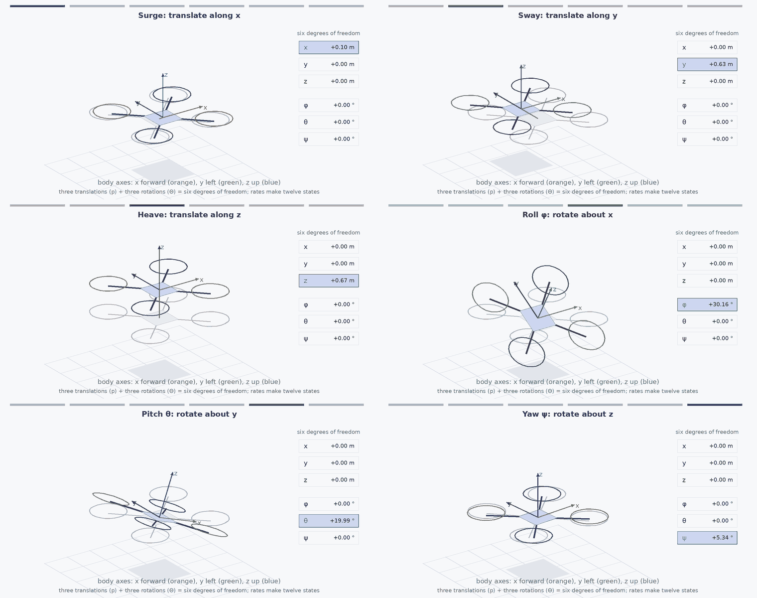
A rigid body in space has six degrees of freedom: three of position and three of orientation. With their rates, the state has twelve numbers: position (3), velocity (3), attitude (roll, pitch, yaw or a quaternion) and body angular rate .
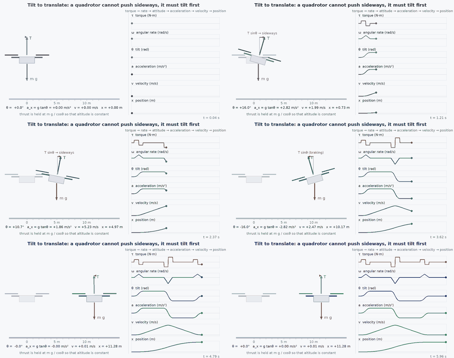
A quadrotor has only four inputs: the four motor thrusts, equivalently a total thrust and three body torques , , . Six degrees of freedom driven by four inputs makes it underactuated: it cannot accelerate sideways directly. To move horizontally it must first tilt, so that part of the thrust points sideways.
Engineering intuition
Think of the vehicle as a thrust vector attached to a rotating platform. Translation is fast to understand: weight pulls down, thrust pushes along the body axis. Rotation is the slow, delicate part: torques from differential thrust change , changes orientation, orientation redirects thrust.
This chain, torque → angular rate → attitude → thrust direction → acceleration → velocity → position, is why controllers are cascaded. Each stage is an integrator or two away from the next. The inner (attitude) loop must be several times faster than the outer (position) loop, otherwise the outer loop sees a lagging plant and oscillates. You can see that in the Quadrotor Dynamics Simulator when the position gains are raised.
Mathematical formulation
Translation (world frame, z up)
Why is the weight term negative?
The weight is not negative: its size is the positive number (14.7 for a 1.5 kg vehicle). The sign gives its direction. Here the world frame has pointing up and is the unit vector along it. Gravity pulls down, opposite to ẑ, so the weight force vector is
On the vertical axis, level thrust gives +T and weight gives −mg, so : the vehicle climbs if > mg, hovers if = mg and sinks if < mg. In a z-down frame such as NED, points down, so the same weight is written +mg and thrust − ; the physics is identical and only the sign convention changes. The code below uses up, which is why it subtracts .
Rotation (body frame)
- ,
- position and velocity in the world frame (, m/s).
- rotation matrix from body to world (lesson M1-T4).
- total thrust, .
- inertia matrix, usually diagonal for a symmetric airframe (kg·).
- angular velocity of the body in the body frame (rad/s).
- torques about the body axes (·), produced by differential motor thrust (lesson M1-T6).
- × J
- gyroscopic term: small for a symmetric vehicle at modest rates.
The Euler kinematics for the ZYX convention, with , are:
The term is the gimbal-lock singularity at ; avoid Euler angles for integration in real flight code.
Hover and small-angle behaviour
At hover, and attitude is level, so . For small angles the horizontal accelerations are and (with forward, left, up), which is the link the position controller uses to turn a desired acceleration into a desired tilt.
Architecture and data flow
In a flight stack the model appears three times, each time with different fidelity:
- Simulator: full nonlinear model with motor dynamics, drag and wind (this lesson).
- Controller design: a linearisation about hover (lesson M5-T7 uses it for LQR) or a simplified point-mass for MPC (lesson M5-T8).
- Estimator: the IMU is treated as measuring and specific force, and the model is used for prediction (module 3).
Real-world UAV applications
- Choosing motors and batteries: and the margin for manoeuvres follow from this model.
- Simulation-first controller tuning before the first flight.
- Predicting how payload mass and centre-of-mass offsets change hover trim.
- Model-based estimation and model predictive control of aggressive flight.
Implementation example
This runs as shown: it integrates the translation and rotation equations from rest, checks that hover thrust keeps the vehicle still, and that zero thrust gives a free fall of ½ .
import numpy as np
g = 9.81

def rot(phi, th, psi):
    cp, sp, ct, st, cy, sy = np.cos(phi), np.sin(phi), np.cos(th), np.sin(th), np.cos(psi), np.sin(psi)
    return np.array([[cy*ct, cy*st*sp - sy*cp, cy*st*cp + sy*sp],
                     [sy*ct, sy*st*sp + cy*cp, sy*st*cp - cy*sp],
                     [-st,   ct*sp,            ct*cp]])

def step(x, T, tau, m, J, dt):
    """x = [p(3), v(3), euler(3), omega(3)], z up. Semi-implicit Euler."""
    p, v, e, w = x[0:3], x[3:6], x[6:9], x[9:12]
    a = rot(*e) @ np.array([0, 0, T]) / m - np.array([0, 0, g])
    wdot = np.linalg.solve(J, tau - np.cross(w, J @ w))
    v = v + a * dt
    p = p + v * dt
    w = w + wdot * dt
    phi, th = e[0], e[1]
    W = np.array([[1, np.sin(phi) * np.tan(th), np.cos(phi) * np.tan(th)],
                  [0, np.cos(phi), -np.sin(phi)],
                  [0, np.sin(phi) / np.cos(th), np.cos(phi) / np.cos(th)]])
    e = e + (W @ w) * dt
    return np.concatenate([p, v, e, w])

m, J, dt = 1.5, np.diag([0.0096, 0.0096, 0.018]), 0.002
x = np.zeros(12)
for _ in range(1000):                       # hover for 2 s: T = m g, no torque
    x = step(x, m * g, np.zeros(3), m, J, dt)
assert np.allclose(x[0:3], 0, atol=1e-9)

x = np.zeros(12)
for _ in range(500):                        # free fall for 1 s
    x = step(x, 0.0, np.zeros(3), m, J, dt)
print("fell", round(-x[2], 3), "m; analytic 0.5*g*t^2 =", round(0.5 * g, 3))
assert abs(-x[2] - 0.5 * g) < 0.02

x = np.zeros(12); x[6] = 0.2                # 0.2 rad roll with hover thrust: it accelerates sideways
for _ in range(100):
    x = step(x, m * g, np.zeros(3), m, J, dt)
assert x[4] < 0                             # roll right-wing-down in z-up/y-left pushes toward -y
print("lateral velocity after 0.2 s:", round(x[4], 3), "m/s")Common engineering mistakes
Forgetting the thrust direction changes with attitude
Using along world . Thrust is along the body axis; only at level attitude is it vertical, and holding altitude while tilted needs .
Using degrees inside trig functions or rates
Equations assume radians everywhere; mixing degrees silently scales torques and angles.
Assuming a point mass is enough for control tuning
Attitude dynamics and motor lag set the achievable bandwidth. A point-mass model is only valid for an outer loop that is much slower than the inner one.
Integrating Euler angles near ±90° pitch
The term blows up; use quaternions.
Using inertia guessed from mass
Inertia scales with mass distribution, not mass. Measure it (bifilar pendulum) or take it from CAD before tuning.
Failure modes
| Failure mode | How it shows up | Likely cause |
|---|---|---|
| Model–vehicle mismatch in inertia | Controller gains that were stable in simulation oscillate on hardware | Inertia, motor lag or thrust coefficient differ from the model |
| Missing motor dynamics | Aggressive attitude commands overshoot on the real vehicle but not in the simulator | Motor/ESC lag adds phase delay that the model omitted |
| Euler-angle singularity | Attitude estimate jumps near vertical flight | Gimbal lock in the Euler kinematics |
| Wrong sign of a torque axis | Roll command pitches the vehicle or the vehicle flips on takeoff | Mixer or frame convention error (lesson M1-T4, M1-T6) |
Debugging approach
- Test the model alone first: hover thrust must keep it still and zero thrust must fall at .
- Apply a small constant roll torque and check the sign and magnitude of the resulting angular acceleration against .
- Compare simulated and logged step responses of attitude: the time constant and overshoot reveal missing lag.
- Check energy: with no thrust and no drag, kinetic plus potential energy must be conserved to integration accuracy.
Practical exercises
- Derive the thrust needed to hold altitude at roll and explain why a vehicle with cannot do it.
- Linearise the model about hover and show that , , and .
- Add linear drag − to the code and find the terminal speed in free fall for .
- Replace Euler angles by a quaternion integration and compare after a pitch manoeuvre.
Interview questions
Write an answer in your own words, then reveal the model answer. Nothing is sent anywhere.
Question 1
Why is a quadrotor underactuated, and how does it translate horizontally?
Model answer
It has four inputs (total thrust and three torques) but six degrees of freedom. It cannot produce horizontal force directly; it tilts so the thrust vector has a horizontal component, which is why attitude control sits inside position control.
Question 2
What is the hover condition?
Model answer
Level attitude and total thrust equal to weight, , with zero angular rate. Tilted, the vertical component must still equal weight, so .
Question 3
Why must the attitude loop be faster than the position loop?
Model answer
The position loop commands tilt; if attitude responds slowly, the position loop sees a delayed plant and loses phase margin. A common rule of thumb is a several-times bandwidth separation.
References and further reading
Primary papers, official documentation and standards. Each claim above that is specific to a tool or version points here.
- R. Mahony, V. Kumar, P. Corke, “Multirotor aerial vehicles: modelling, estimation and control of quadrotor”, IEEE RAM, 2012
- D. Mellinger, V. Kumar, “Minimum snap trajectory generation and control for quadrotors”, ICRA 2011 (model and differential flatness)
- PX4 documentation: multicopter control architecture