UAV Systems Engineering · Module 8
M8-T6: Test-case development
A test case is an experiment: it fixes what you do, what you expect, and how you decide, before you look at the data.
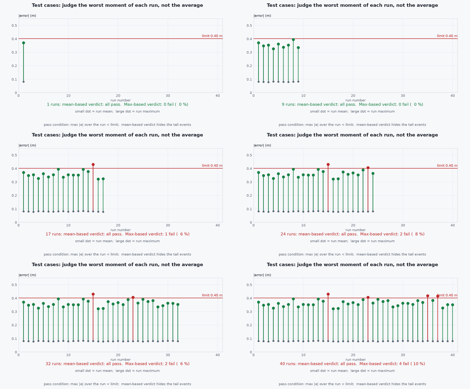
Good test cases share one trait: the verdict is decided by a rule written before the run. That requires preconditions, a stimulus that can be repeated, a numerical criterion, a statistic and a number of repetitions that supports it. For a navigation system the most valuable cases inject faults, because nominal operation tells you little about safety.
Learning objectives
After this lesson, you should be able to:
- Write a complete test case with preconditions, stimulus, expected result, criterion, repetitions and evidence.
- Design fault-injection stimuli for sensors and links and know the injection points.
- Choose pass criteria that use the right statistic and sample size.
- Implement a test case as an executable, seeded, deterministic regression test.
Conceptual explanation
Established The structure is standard in software and systems testing. The example scenario uses a toy estimator to illustrate the method: it is not a model of any particular flight stack.
A test case has seven parts:
| Part | Content | Example |
|---|---|---|
| ID and traced requirement | Link to the requirement it verifies | T-101 verifies R-10 |
| Preconditions | Baseline, configuration, vehicle state, environment | Baseline v1.4, VIO fused, hover at 3 m, lit scene |
| Stimulus | Scenario and injected faults, with times | Disable GNSS at ; fly a 20 m square; blank the camera for 2 s at |
| Observations | Signals recorded, rates, reference source | Estimate, reference trajectory, innovations, mode |
| Expected result and criterion | Quantity, threshold, statistic | p95 horizontal error ≤ 2 m over the segment |
| Repetitions | Number of runs and seeds or trials | 45 runs with different seeds |
| Verdict rules | Pass, fail, and invalid (test did not execute as specified) | Invalid if the reference is missing for > 1 s |
Fault injection places a fault at a defined point in the data path: in the simulator (sensor model), between driver and consumer (a wrapper that drops, freezes or corrupts messages), in the network (delay, loss), or physically (disconnecting a cable on the ground). Choose fault types from the FMEA: dropout, freeze (stuck value), bias step, noise increase, delay, saturation, wrong frame.
Engineering intuition
The temptation after a run is to look at the plot and decide whether it “looks okay”. A written criterion removes that bias. It also protects you from the opposite problem: a result that looks bad but meets the criterion (noise in a plot) or that looks good but fails it on the tail. The “invalid” verdict matters as much as pass and fail: a run in which the reference system dropped out proves nothing and must not count toward either.
Seed everything random and record the seed with the result. A failure you cannot reproduce cannot be fixed; a failure with a seed becomes a unit test.
Mathematical formulation
For a continuous error metric the pass criterion is usually on a percentile of the error over runs or time. To verify “the 95th percentile of the error is below L” with confidence from independent run-level maxima or run-level metrics, count the runs exceeding : the claim is supported if the number of exceedances is small enough that the Clopper-Pearson upper bound on the exceedance probability is below 5 %:
For this needs trials (45 at , 59 at ). A metric defined per sample (error at 10 Hz for 5 minutes) has strongly correlated samples: the effective sample size is much smaller than the sample count, so use a run-level statistic or a block bootstrap, not the raw count. For fault-detection requirements (“detect within 0.5 s”) the criterion is on the detection delay distribution and on the probability of detection, with a false-alarm limit measured over fault-free runs.
- significance level.
- ,
- number of exceedances and of runs.
- error threshold in the requirement.
Architecture and data flow
Test case file (YAML) → harness (SIL/HIL runner or flight card) → baseline loaded and verified → scenario with seeded fault injection → recorded logs → analysis function computing the metric → verdict logic (pass, fail, invalid) → result record with baseline ID, seed, data pointer → traceability matrix. In CI, the same harness runs a reduced set per commit and the full set per release.
Real-world UAV applications
- Verifying the GNSS-loss failsafe timing.
- Verifying drift bounds under VIO degradation.
- Regression tests that catch estimator behaviour changes.
- Fault-injection campaigns derived from the FMEA.
Implementation example
This runs as shown. An executable test case: a 1D position estimator (a Kalman filter fusing GNSS position and a drifting odometry velocity), a seeded GNSS-dropout injection, and a verdict function with a run-level p95 criterion, an invalid-run rule and the zero-failure sample size. The toy estimator stands in for the system under test.
import numpy as np, math

def run_case(seed, drop_at=30.0, T=120.0, dt=0.1, vo_bias_sd=0.01):
    rng = np.random.default_rng(seed); n = int(T / dt); x_true = 0.0; v = 1.0
    xh = np.array([0.0, v]); P = np.diag([1.0, 0.1]); F = np.array([[1, dt], [0, 1]]); Q = np.diag([1e-4, 1e-4]) * dt
    vo_bias = rng.normal(0, vo_bias_sd); err = []; ref_ok = True
    for k in range(n):
        t = k * dt; x_true += v * dt
        xh = F @ xh; P = F @ P @ F.T + Q
        if t < drop_at and k % 10 == 0:                                 # GNSS at 1 Hz, until the injected dropout
            H = np.array([[1.0, 0.0]]); S = H @ P @ H.T + 4.0; K = P @ H.T / S
            xh = xh + (K * (x_true + 2.0 * rng.standard_normal() - xh[0])).ravel(); P = (np.eye(2) - K @ H) @ P
        if k % 2 == 0:                                                  # visual odometry velocity at 5 Hz, with a constant bias
            H = np.array([[0.0, 1.0]]); S = H @ P @ H.T + 0.05 ** 2; K = P @ H.T / S
            xh = xh + (K * (v + vo_bias + 0.05 * rng.standard_normal() - xh[1])).ravel(); P = (np.eye(2) - K @ H) @ P
        if t >= drop_at: err.append(abs(xh[0] - x_true))
    return np.array(err), ref_ok
def verdict(errs, L=3.0, req_p=0.95, alpha=0.10):
    # run-level metric: the maximum error in the denied segment; criterion: <= L in at least req_p of runs (zero-failure demonstration)
    n_needed = math.ceil(math.log(alpha) / math.log(req_p)); maxima = np.array([e.max() for e in errs])
    x = int((maxima > L).sum())
    if len(errs) < n_needed: return 'INVALID (too few runs: need %d)' % n_needed, maxima
    return ('PASS' if x == 0 else 'FAIL (%d of %d runs exceeded %.1f m)' % (x, len(errs), L)), maxima
runs = [run_case(s)[0] for s in range(45)]
v1, maxima = verdict(runs)
print(f"45 runs: median of run maxima {np.median(maxima):.2f} m, worst {maxima.max():.2f} m -> {v1}")
v2, _ = verdict(runs[:20]); print("20 runs ->", v2)
assert v2.startswith('INVALID') and math.ceil(math.log(0.10) / math.log(0.95)) == 45
v3, _ = verdict([run_case(s, vo_bias_sd=0.2)[0] for s in range(45)]); print("with a larger odometry bias (0.2 m/s sd):", v3)
assert v1 == 'PASS' and v3.startswith('FAIL')Common engineering mistakes
Deciding the criterion after seeing the data
Write the pass rule before the run.
Using raw sample counts for correlated data
Effective sample size is far smaller; use run-level metrics or block statistics.
No invalid verdict
Runs where the reference or logging failed must not count.
Unseeded fault injection
A failure that cannot be replayed is hard to fix.
Only nominal cases
The value is in faults and edges; derive them from the FMEA.
Failure modes
| Failure mode | How it shows up | Likely cause |
|---|---|---|
| Flaky test | Passes and fails at random | Unseeded randomness or timing dependence |
| False confidence | Passes with few runs | Sample size below what the statistic needs |
| Undetected defect | Failure not covered | No fault-injection case for that failure mode |
| Disputed verdict | Argument over a borderline run | Criterion or statistic not specified |
Debugging approach
- Re-run the failing seed with logging on and plot the estimate against the reference.
- Check the preconditions that were actually met against those specified.
- Compare run-level metrics between baselines to spot regressions.
- Review injected faults against the FMEA for coverage.
Practical exercises
- Write the test case table for a VIO dropout of 2 s with a detection-time requirement of 0.5 s.
- Compute the number of runs for 99 % at 90 % confidence with zero failures.
- Extend the example with a 10 s GNSS spoof (a constant 5 m offset) and decide the criterion.
- Add an invalid-run rule for missing reference data.
Interview questions
Write an answer in your own words, then reveal the model answer. Nothing is sent anywhere.
Question 1
What is the difference between fail and invalid?
Model answer
Fail means the system did not meet the criterion in a correctly executed test; invalid means the test did not execute as specified (missing reference, wrong baseline), so it says nothing about the system and must be rerun.
Question 2
Why not count every sample toward the statistics?
Model answer
Samples in a time series are strongly correlated, so the effective sample size is much smaller; use run-level metrics or block methods for the sample size.
Question 3
Why seed fault injection?
Model answer
To reproduce failures exactly, turn them into regression tests and attribute differences to code changes rather than chance.
References and further reading
Primary papers, official documentation and standards. Each claim above that is specific to a tool or version points here.