UAV Systems Engineering · Module 5
M5-T17: 3-D path planning on voxel maps
Planning in the air is the same search as on the ground with one more axis, and that axis costs a factor of eight in cells every time you halve the cell size.
A UAV moves in three dimensions, so its planner searches a three-dimensional map. The algorithm is the A* of the previous planning lesson, but the neighbours, the step costs, the heuristic, the memory and the safety margins all change with the extra axis. This lesson builds the 3-D version, shows what the heuristic buys, and explains how the resolution of the map and the inflation of obstacles decide both the cost of the search and the safety of the result.
Learning objectives
After this lesson, you should be able to:
- Describe a 3-D voxel map and compare a dense grid, an octree and a distance field as map representations.
- Write the 26-neighbour step costs and the 3-D octile heuristic, and explain why the heuristic is admissible and consistent.
- Choose the map resolution and the obstacle inflation from the vehicle size, and predict how the search cost scales with the cell size.
- Shorten a grid path with line-of-sight checks and state what the back end of the planner must still do.
Conceptual explanation
Established A* (Hart, Nilsson and Raphael, 1968), occupancy grids and octrees (for example OctoMap) and any-angle shortcuts are standard techniques. The map, the numbers of cells and expansions and the margins below are illustrative values from the example in this lesson, not properties of a particular vehicle or sensor.
A voxel map divides space into cubes of side and stores, for each cube, whether it is free, occupied or unknown. It is the three-dimensional occupancy grid that LiDAR or depth-camera mapping produces (Module 4). A planner treats each free cube as a node and connects it to its neighbours.
In 2-D a cell has 8 neighbours. In 3-D it has 26: 6 across faces, 12 across edges and 8 across corners, with step lengths of 1, and cells. That changes three things in the planner:
- Step costs are the Euclidean lengths of the moves, so a corner move costs , not 1.
- The heuristic must use all three axes: the 3-D octile distance below.
- Memory and time grow with the cube of the resolution. A map ten times finer has a thousand times more cells.
The map can be stored in three common ways:
| Representation | Idea | Good for | Cost |
|---|---|---|---|
| Dense voxel grid | One value per cube in a 3-D array | Fast lookups and simple planners; local maps around the vehicle | Memory ∝ volume ÷ , even for empty space |
| Octree (for example OctoMap) | Recursively split a cube into eight; keep large cubes where space is uniform | Large environments at fine resolution; probabilistic occupancy | Pointer-based, slower to query than an array |
| Distance field (ESDF) | Store the distance from each cell to the nearest obstacle | Clearance checks, gradient-based smoothing, safe-corridor construction | Must be updated as the map changes |
Two decisions in the map decide whether the plan is safe. Unknown space is usually treated as an obstacle when flying in an unmapped environment, and as free only when the mission is exploration with a reactive layer behind the planner. Altitude is not free: the vehicle has a ceiling and a floor, climbing costs energy, and an optimal path may be allowed to go over an obstacle, which a 2-D planner could never do.
Engineering intuition
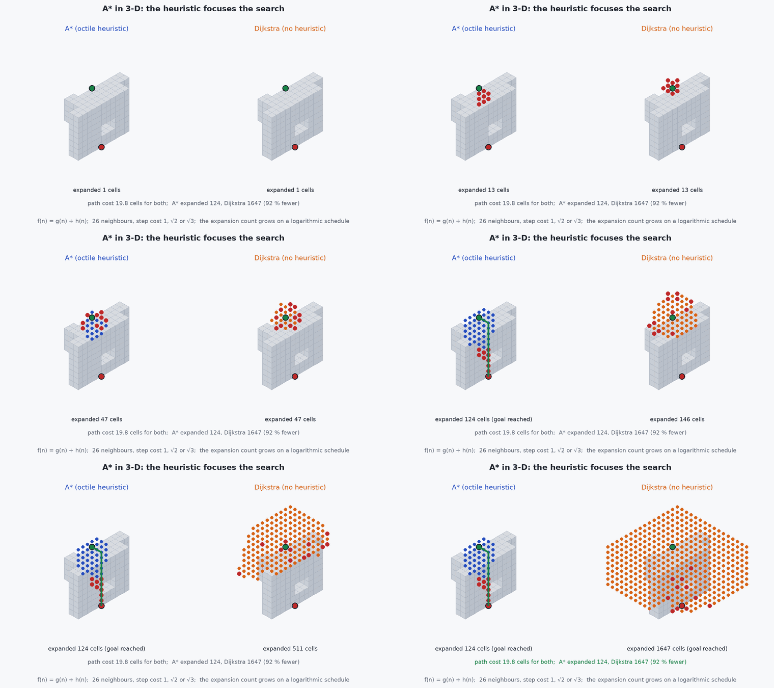
Picture a three-dimensional maze made of cubes. A* explores like a flood of water that is pulled towards the goal: it expands the cells that look cheapest overall, the cost so far plus an optimistic estimate of the cost to go. With no estimate (Dijkstra’s algorithm) the flood spreads evenly in every direction, including away from the goal, and fills most of the free space before it arrives. The estimate costs nothing to compute and, in this lesson’s example, cuts the work by more than ten times.
The grid path is the cheapest sequence of cells, not the shortest curve. It turns in multiples of and often zig-zags. A shortcut that checks straight lines between waypoints removes most of that, but a straight line can pass close to a corner of an obstacle, so the check has to use the inflated map. And the finer the grid, the better the path and the longer the search, so the resolution is a trade between path quality and planning time, set by how fast the vehicle must replan.
Mathematical formulation
Cost and heuristic
A* expands the node with the smallest estimated total cost, the cost accumulated from the start plus an estimate of the remaining cost:
Moving between two neighbouring cell centres costs their distance in cells:
On an empty grid the cheapest way to cover offsets of cells along the three axes (sorted) is corner moves, then edge moves, then straight moves. Its cost is the 3-D octile distance:
Obstacles can only make the true cost larger, so never overestimates (it is admissible). It also satisfies for every move (it is consistent), so A* never needs to reopen a cell and returns an optimal path. A weighted version, with , expands fewer cells at the price of a path at most times longer than optimal.
Resolution, memory and safety
For a region of size the number of cells, and therefore the memory of a dense grid, scales with the inverse cube of the cell size:
For example a 100 m × 100 m × 30 m region at has cells (2.4 MB at one byte per cell), and at it has cells (300 MB). Because the search expands cells on a surface that also grows with resolution, the work grows by a similar factor per halving.
The vehicle is not a point. An obstacle surface can lie anywhere inside an occupied cell, and a path through free cell centres can pass anywhere within half a cell of them. A conservative inflation radius is therefore
- cell size (m).
- , ,
- cells of the grid.
- , ,
- cost so far, heuristic estimate, and their sum.
- sorted absolute offsets to the goal, in cells.
- ,
- vehicle radius and safety margin (m).
Architecture and data flow
The planner reads the current voxel map (and its distance field) from the mapping module (Module 4) and the vehicle state from the estimator. It inflates the map, searches from the current position to the goal, shortens the path with line-of-sight checks on the inflated map, and passes the few remaining waypoints to the trajectory generator (lesson M5-T9), which builds a smooth polynomial through them within the velocity and acceleration limits (lesson M5-T12). The tracking controller (lesson M5-T14) flies the result. When the map changes, a monitor checks the remaining trajectory for collision and triggers a replan; the sensing and planning latency set how fast the vehicle may fly (lesson M5-T13).
Real-world UAV applications
- Global planning for a UAV that flies through a mapped building, tunnel or forest.
- Replanning around newly sensed obstacles in a local voxel map around the vehicle.
- Inspection paths that go over, around or through openings in structures.
- Generating a topologically correct initial path for a smoothing or corridor-based optimiser.
Implementation example
This runs as shown. It builds a 16 × 16 × 8 voxel map with a low wall, a full-height wall with a window and a pillar, and runs 26-connected A* with the 3-D octile heuristic. The tests check that A* finds the same optimal cost as Dijkstra’s algorithm with far fewer expansions, that the path is collision-free and never shorter than the straight line, that the heuristic is consistent, that inflation keeps the clearance, that the shortcut path is shorter and clear, and that halving the cell size multiplies the cells by eight and the work by much more.
import heapq, math
import numpy as np

def make_world(scale=1):
    """A 16 x 16 x 8 voxel map (times `scale` per axis): a low wall, a full-height wall with a window, and a pillar."""
    occ = np.zeros((16, 16, 8), bool)
    occ[5:7, 0:11, 0:5] = True          # low wall: go over it (z >= 5) or around it (y >= 11)
    occ[10:12, 5:16, :] = True          # full-height wall ...
    occ[10:12, 8:11, 2:4] = False       # ... with a window (y 8..10, z 2..3)
    occ[3:5, 8:10, 0:4] = True          # pillar
    return np.repeat(np.repeat(np.repeat(occ, scale, 0), scale, 1), scale, 2)

N26 = [(i, j, k) for i in (-1, 0, 1) for j in (-1, 0, 1) for k in (-1, 0, 1) if (i, j, k) != (0, 0, 0)]

def h_oct3(a, b):
    """3-D octile distance in cells: exact cost of the best path on an empty 26-connected grid."""
    d = sorted(abs(a[i] - b[i]) for i in range(3))
    return (math.sqrt(3) - math.sqrt(2)) * d[0] + (math.sqrt(2) - 1) * d[1] + d[2]

def inflate(occ, r):
    """Block every cell whose centre is within r cells of an occupied cell (spherical dilation)."""
    out = occ.copy(); R = int(math.ceil(r))
    for dx in range(-R, R + 1):
        for dy in range(-R, R + 1):
            for dz in range(-R, R + 1):
                if dx * dx + dy * dy + dz * dz <= r * r and (dx, dy, dz) != (0, 0, 0):
                    src = occ[max(0, -dx):occ.shape[0] - max(0, dx), max(0, -dy):occ.shape[1] - max(0, dy), max(0, -dz):occ.shape[2] - max(0, dz)]
                    out[max(0, dx):occ.shape[0] - max(0, -dx), max(0, dy):occ.shape[1] - max(0, -dy), max(0, dz):occ.shape[2] - max(0, -dz)] |= src
    return out

def astar(occ, s, g, use_h=True):
    """A* on a 26-connected grid. Returns (path, cost, number of expanded cells)."""
    shape = occ.shape; openq = [(h_oct3(s, g) if use_h else 0.0, 0.0, s)]; gs = {s: 0.0}; parent = {s: None}; closed = set()
    while openq:
        _, gc, u = heapq.heappop(openq)
        if u in closed: continue
        closed.add(u)
        if u == g: break
        for d in N26:
            v = (u[0] + d[0], u[1] + d[1], u[2] + d[2])
            if not all(0 <= v[i] < shape[i] for i in range(3)) or occ[v] or v in closed: continue
            ng = gc + math.sqrt(d[0] ** 2 + d[1] ** 2 + d[2] ** 2)          # 1, sqrt 2 or sqrt 3
            if ng < gs.get(v, 1e18): gs[v] = ng; parent[v] = u; heapq.heappush(openq, (ng + (h_oct3(v, g) if use_h else 0.0), ng, v))
    if g not in parent: return None, None, len(closed)
    path = []; u = g
    while u is not None: path.append(u); u = parent[u]
    return path[::-1], gs[g], len(closed)

def clear_segment(occ, a, b, step=0.25):
    """Line of sight between two cell centres: sample the segment and test the voxel under every sample."""
    a, b = np.array(a, float) + 0.5, np.array(b, float) + 0.5; n = max(1, int(np.linalg.norm(b - a) / step))
    return all(not occ[tuple(np.floor(a + (b - a) * t / n).astype(int))] for t in range(n + 1))

def shortcut(occ, path):
    """Greedy any-angle shortcut: from each waypoint jump to the farthest waypoint that is still in line of sight."""
    out = [path[0]]; i = 0
    while i < len(path) - 1:
        j = len(path) - 1
        while j > i + 1 and not clear_segment(occ, path[i], path[j]): j -= 1
        out.append(path[j]); i = j
    return out

length = lambda pts: sum(math.dist(pts[i], pts[i + 1]) for i in range(len(pts) - 1))

occ = make_world(); s, g = (1, 2, 1), (14, 13, 2)
path, cost, n_a = astar(occ, s, g)
p0, cost0, n_d = astar(occ, s, g, use_h=False)                       # Dijkstra: the same search with h = 0
print(f"A*: cost {cost:.2f}, {n_a} expansions;  Dijkstra: cost {cost0:.2f}, {n_d} expansions")
assert abs(cost - cost0) < 1e-9 and n_a < n_d                         # same optimal cost, fewer expansions
assert not any(occ[c] for c in path) and all(max(abs(path[i + 1][k] - path[i][k]) for k in range(3)) == 1 for i in range(len(path) - 1))
assert cost >= math.dist(s, g) - 1e-9                                 # never shorter than the straight line

rs = np.random.default_rng(1); free = [tuple(c) for c in np.argwhere(~occ)]
for _ in range(2000):                                                 # consistency: h(u) <= c(u, v) + h(v) for every neighbour
    u = free[rs.integers(len(free))]; d = N26[rs.integers(26)]; v = (u[0] + d[0], u[1] + d[1], u[2] + d[2])
    assert h_oct3(u, g) <= math.sqrt(sum(x * x for x in d)) + h_oct3(v, g) + 1e-9

r = 1.5                                                               # vehicle radius plus margin, in cells
occ_i = inflate(occ, r); pi, ci, _ = astar(occ_i, s, g)
obst = np.argwhere(occ); clearance = min(np.min(np.linalg.norm(obst - np.array(c), axis=1)) for c in pi)
print(f"inflated by {r} cells: cost {ci:.2f}, minimum clearance {clearance:.2f} cells")
assert ci >= cost - 1e-9 and clearance > r                            # a larger robot never finds a shorter path and keeps its clearance

sc = shortcut(occ_i, pi)
print(f"waypoints {len(pi)} -> {len(sc)}, length {length(pi):.2f} -> {length(sc):.2f} cells")
assert len(sc) < len(pi) and length(sc) <= length(pi) + 1e-9
assert all(clear_segment(occ_i, sc[i], sc[i + 1]) for i in range(len(sc) - 1))

fine = make_world(2); sf, gf = tuple(2 * x for x in s), tuple(2 * x for x in g)
_, cf, n_f = astar(fine, sf, gf)
print(f"cells {occ.size} -> {fine.size} (x{fine.size // occ.size});  A* expansions {n_a} -> {n_f}")
assert fine.size == 8 * occ.size and n_f > 3 * n_a # halving the cell size multiplies the cells by 8 and the work by a lotThe animation in the concept section runs the same two searches on the same map.
Common engineering mistakes
Using the 2-D octile heuristic or the Manhattan distance in 3-D
A heuristic that overestimates breaks optimality; one that ignores an axis gives up the speed-up. Use the 3-D octile distance for a 26-connected grid.
Planning through cell centres with no inflation
The path touches obstacle corners. Inflate by the vehicle radius, a margin and the half-diagonal of a cell, and check shortcuts on the inflated map.
Treating unknown space as free
The plan flies into places the sensors have not seen. In an unmapped environment treat unknown as occupied, or keep a reactive layer that can stop the vehicle.
Choosing the finest resolution the sensor can give
Cells and search work grow with the cube of the resolution, so the planner is too slow to replan. Choose the coarsest that keeps narrow gaps open.
Flying the grid path directly
It turns in multiples of and zig-zags, which demands acceleration the vehicle does not have. Shorten it and pass it through a trajectory generator.
Failure modes
| Failure mode | How it shows up | Likely cause |
|---|---|---|
| Planner finds no path | Search exhausts the map and returns nothing | Inflation closed a narrow opening, or the start or goal lies inside the inflated obstacles |
| Plan takes too long to replan | Planning time exceeds the replanning period | Map too fine for the region, or the search area is not limited to a local window |
| Vehicle clips an obstacle corner | Contact or near miss at a corner | Inflation without the half-diagonal term, tracking error larger than the margin, or a shortcut checked on the uninflated map |
| Path climbs and descends unnecessarily | Altitude oscillates along the route | Step costs treat vertical and horizontal moves alike with no penalty or limit on climbing |
Debugging approach
- Draw the inflated map next to the original and check that known openings are still open.
- Run Dijkstra and compare the cost with A*: any difference means the heuristic is not admissible.
- Count expansions as the cell size changes and compare with the factor of eight per halving.
- Check each shortcut segment against the inflated map, not the raw map, and log the minimum clearance along the path.
Practical exercises
- Show that the 3-D octile distance equals the cost of the best path on an empty 26-connected grid, by counting moves for the offset (3, 5, 9).
- Add a vertical-move penalty of 1.5 to the step cost and observe the change in the path; what happens to the admissibility of the heuristic?
- Change the weight to and plot the expansions and the path cost against ; compare with the bound of times the optimal cost.
- Downsample the map by two with an any-occupied rule and plan again; find a window size at which the path is lost.
Interview questions
Write an answer in your own words, then reveal the model answer. Nothing is sent anywhere.
Question 1
What changes when you move A* from 2-D to 3-D?
Model answer
Each cell has 26 neighbours instead of 8, with step costs of 1, and , the heuristic uses all three axes (the 3-D octile distance), and memory and search effort grow with the cube of the resolution, so the map resolution becomes a main design choice.
Question 2
Why is the 3-D octile distance an admissible heuristic?
Model answer
It is the exact cost of the best path on an empty grid with the same moves, and obstacles can only add cost, so it never overestimates the true cost. It is also consistent, so A* returns an optimal path without reopening cells.
Question 3
Why inflate by more than the vehicle radius?
Model answer
An obstacle surface can lie anywhere inside an occupied cell and a path through cell centres can deviate by up to half a cell diagonal, so the clearance must also cover the cell resolution and the vehicle’s tracking and localisation error. The radius alone would leave no margin.
References and further reading
Primary papers, official documentation and standards. Each claim above that is specific to a tool or version points here.
- P. E. Hart, N. J. Nilsson, B. Raphael, “A formal basis for the heuristic determination of minimum cost paths”, IEEE Transactions on Systems Science and Cybernetics, 1968
- A. Hornung et al., “OctoMap: an efficient probabilistic 3D mapping framework based on octrees”, Autonomous Robots, 2013
- K. Daniel, A. Nash, S. Koenig, A. Felner, “Theta*: any-angle path planning on grids”, Journal of Artificial Intelligence Research, 2010 (line-of-sight shortcuts inside the search)
- S. Karaman, E. Frazzoli, “Sampling-based algorithms for optimal motion planning”, International Journal of Robotics Research, 2011 (RRT* in continuous 3-D space)
- S. Liu et al., “Planning dynamically feasible trajectories for quadrotors using safe flight corridors in 3-D complex environments”, IEEE Robotics and Automation Letters, 2017
- B. Zhou et al., “Robust and efficient quadrotor trajectory generation for fast autonomous flight”, IEEE Robotics and Automation Letters, 2019