UAV Systems Engineering · Interactive simulation · M5-L6

3-D Voxel Path Planner

A voxel map, a search and a vehicle with a size: see what the heuristic saves, when it breaks, and when the vehicle no longer fits.

UAV Guidance, Navigation and Control (GNC)
Established engineering
Runs entirely in your browser

What you are looking at

The map is a 16 × 16 × 8 grid of cubes (cells): a low wall you can fly over or around, a full-height wall with a window, and a pillar. The planner searches from the green cell to the red cell. Blue dots are the cells the search expanded (the last few in red while the search plays), the green line is the path it found, and the orange dashed line is the same path after a line-of-sight shortcut. Orange dots are free cells that the inflation (the vehicle’s radius) has blocked.

The numbers show how many cells A* expanded (and how many Dijkstra’s algorithm would), the path cost in cells, its ratio to the optimal cost, and the number of waypoints before and after the shortcut. The lower plot re-plans for every inflation radius from 0 to 3.5 cells with the current settings and shows where the path cost jumps and where no path exists.

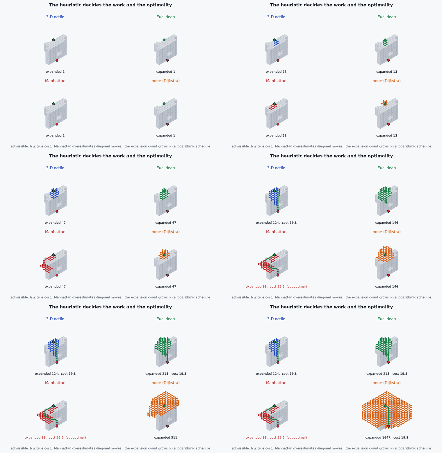
Animation of four searches on the same three-dimensional voxel map, drawn in four isometric panels: A* with the three-dimensional octile heuristic, with the Euclidean heuristic, with the Manhattan heuristic and with no heuristic at all, which is Dijkstra’s algorithm. All four advance together by the same number of expanded cells. The octile heuristic finishes first with the optimal path, the Euclidean heuristic also gives the optimal path but expands more cells, Manhattan expands few cells but returns a longer path because it overestimates the cost of diagonal moves, and the search without a heuristic expands the most. Each panel ends with its count of expanded cells and the path cost. — An admissible heuristic never overestimates, so A* stays optimal; the closer it is to the true cost, the fewer cells are expanded. Manhattan distance is not admissible when diagonal moves are allowed. All four use the 26-connected grid and the same start and goal; the counts come from running the four searches. The expansion count shown grows on a logarithmic schedule. (Looping, about 6 seconds; drawn and computed for this course with illustrative values.)

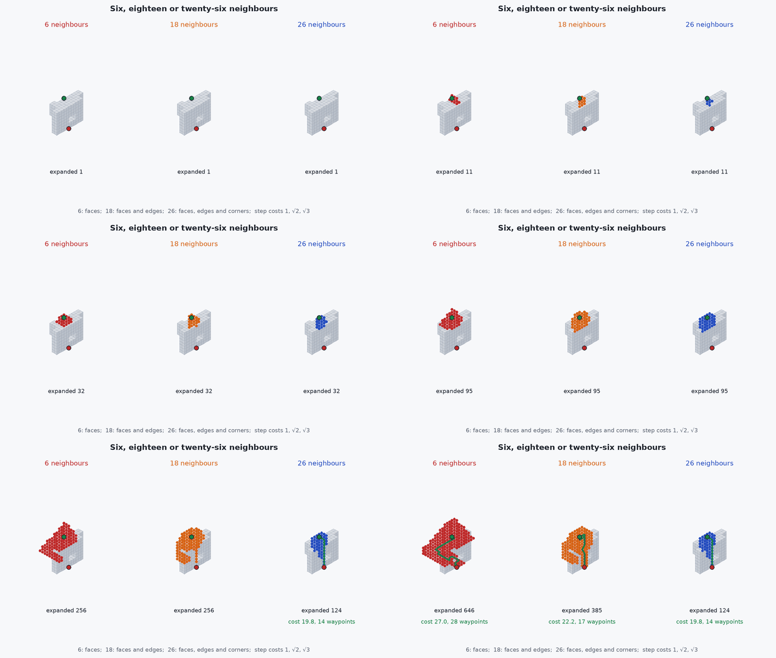
Animation of the same A* search on a three-dimensional voxel map with three neighbour sets, drawn in three isometric panels: six neighbours across the faces of a cell, eighteen neighbours across faces and edges, and twenty-six neighbours across faces, edges and corners. The three searches advance together. With six neighbours the path can only follow the axes and is much longer, with eighteen it is shorter, and with twenty-six it is the shortest; the search with more neighbours expands cells in more directions at each step. Each panel ends with its path cost and the number of waypoints. — More neighbours mean more directions of motion and a path closer to the straight line, at the price of more work per expanded cell. The step costs are the Euclidean lengths 1, √2 and √3, and the heuristic is the 3-D octile distance, which stays admissible for all three sets. The numbers come from running the three searches; the expansion count shown grows on a logarithmic schedule. (Looping, about 6 seconds; drawn and computed for this course with illustrative values.)

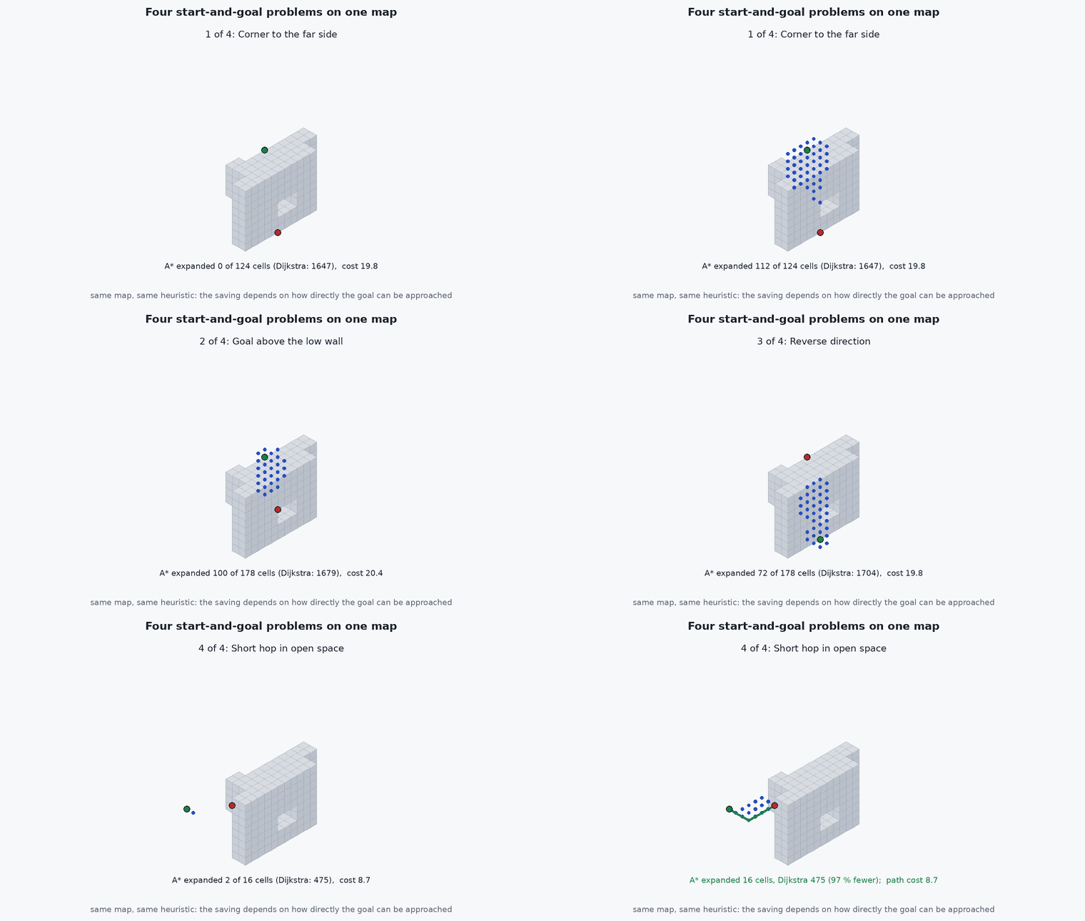
Animation of the four start-and-goal problems offered by the voxel planner simulation, each solved by A* with the three-dimensional octile heuristic on the same map and drawn in isometric view. For each problem the cells expanded by the search appear as blue dots and the resulting path is drawn in green; the problems are a corner-to-far-side flight through the window, a flight to a goal above the height of the low wall, the reverse direction, and a short hop in open space. A counter shows the cells expanded by A* and by Dijkstra’s algorithm and the path cost, and the savings are largest where a straight run towards the goal is blocked. — The same planner, map and heuristic solve all four problems; only the start and the goal change. How much the heuristic saves depends on the problem: it saves most when the goal can be approached directly and least when the search must go around obstacles. The numbers come from running the searches. (Looping, about 5 seconds; drawn and computed for this course with illustrative values.)

Try this

Choose the heuristic “None (Dijkstra)” and compare the cells expanded with the 3-D octile heuristic. The cost is the same; the work is not.
Choose the Manhattan heuristic with 26 neighbours. It overestimates the cost of diagonal moves, so A* is no longer optimal: read the ratio to the optimal cost.
Raise the weight from 1 to 3 and watch the expansions fall and the cost rise, always staying below the weight times the optimum.
Raise the inflation radius from 0 in steps of 0.25. Find the radius at which the path stops going through the window, and the radius at which planning becomes impossible. Is it a route that closes, or the goal cell itself that becomes blocked?

Model and its limits

Included: a voxel map with occupied and free cells, 6, 18 or 26 neighbours with Euclidean step costs, four heuristics (3-D octile, Euclidean, Manhattan, none), a weight on the heuristic, spherical obstacle inflation by cell-centre distance, a binary-heap A* that returns the expansion order, and a line-of-sight shortcut that samples each segment every quarter of a cell.

Not included: unknown space and a map that changes, a distance field, sampling-based planners, vehicle dynamics and any smoothing (the path is a geometric path, not a trajectory a vehicle can fly), and the extra margin for cell size and tracking error that a real inflation radius needs (lesson M5-T17). The map and all numbers are illustrative.

Related lessons

Saved in this browser and synced to your account when you are signed in.

Back to Module 5 · UAV track overview