UAV Systems Engineering · Module 3
M3-T4: Kalman Filter
A Kalman filter is a weighted average whose weights come from honest uncertainty: derive it, run it, and see the gain move.
Every estimator in this track, from the autopilot’s EKF2 to FAST-LIO2, is a Kalman filter or a close relative. The linear case is small enough to derive in full and run in twenty lines, and it explains the behaviour of the rest.
Learning objectives
After this lesson, you should be able to:
- Write the predict and update equations of the Kalman filter and say what each term means.
- Derive the Kalman gain as the minimiser of posterior variance in the scalar case.
- Explain how and set the trade-off between model and measurement.
- Implement a constant-velocity filter and check its consistency.
Conceptual explanation
The Kalman filter keeps a Gaussian belief over the state: a mean and a covariance . It alternates two steps. Predict: push the belief through the motion model; uncertainty grows because the model is imperfect (process noise ). Update: when a measurement arrives, blend it with the prediction; uncertainty shrinks. The blend weight is the Kalman gain .
For linear models with Gaussian noise, it is the exact Bayesian posterior and the minimum-variance linear estimator. For non-linear ones (lesson M3-T5) it is an approximation.
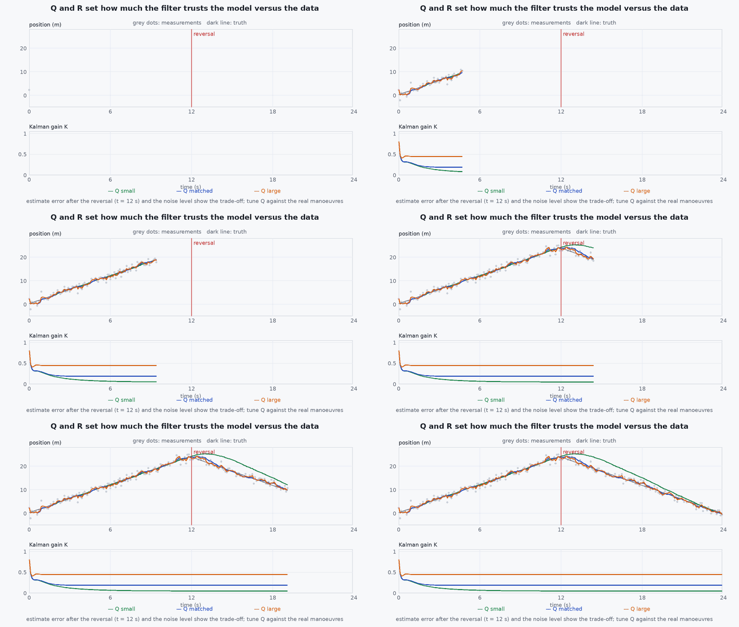
Engineering intuition
In one dimension, the update is a weighted average of the prediction and the measurement, weighted by the inverse of their variances: whichever is more certain gets more weight. ⁻/(⁻ + ) is between 0 and 1: near 0 when the measurement is noisy ( large) and near 1 when the prediction is poor (⁻ large). Tuning is therefore a statement about how much you trust your model: a large makes the filter nervous and responsive, a small makes it smooth and slow to react to real changes.
Mathematical formulation
Model: , ~ (0, ); measurement , ~ (0, ).
- ,
- state estimate and its covariance.
- , ,
- state-transition, input and measurement matrices.
- ,
- process and measurement noise covariances.
- ,
- innovation (residual) and its covariance: used for gating and consistency (lessons M3-T13, M3-T14).
- Kalman gain.
Scalar derivation
Combine a prior (⁻, ⁻) and a measurement with variance . The posterior mean ⁻ + ( − ⁻) has variance ⁻ + . Setting the derivative with respect to to zero:
The posterior is always more certain than either source. The Joseph form shown above is algebraically equal to ( − KH)⁻ but keeps symmetric positive definite under rounding error, so use it in real code.
Constant-velocity model
Architecture and data flow
Sensor sample → timestamp and validity check → predict to the measurement time (never to “now”) → update → publish state and covariance. Getting the time of the prediction right is the most common implementation detail missed in practice: a measurement that is 80 ms old must be applied to the state as it was 80 ms ago, or an out-of-sequence strategy must be used.
Real-world UAV applications
- GNSS-aided position and velocity tracking.
- Altitude estimation from barometer and accelerometer.
- Target tracking for follow-me and landing.
- The core of the EKF inside PX4 and of every VIO and LIO system.
Implementation example
This runs as shown: a constant-velocity filter tracks a vehicle from noisy position measurements; it checks accuracy and that the filter’s covariance matches the actual error (statistical consistency).
import numpy as np
rng = np.random.default_rng(3)
dt, n = 0.1, 400
F = np.array([[1, dt], [0, 1]]); H = np.array([[1.0, 0.0]])
q = 0.5                                            # white acceleration spectral density
Q = q * np.array([[dt**3 / 3, dt**2 / 2], [dt**2 / 2, dt]])
R = np.array([[2.0**2]])                           # 2 m measurement sigma

# truth: accelerations are white noise with the SAME spectral density, so the model is correct
x_true = np.zeros((n, 2)); x = np.array([0.0, 5.0])
L = np.linalg.cholesky(Q)
for k in range(n):
    x = F @ x + L @ rng.standard_normal(2); x_true[k] = x
z = x_true[:, 0] + 2.0 * rng.standard_normal(n)

xh = np.array([0.0, 0.0]); P = np.diag([25.0, 25.0])
nees, err = [], []
for k in range(n):
    xh = F @ xh; P = F @ P @ F.T + Q                       # predict
    y = z[k] - H @ xh; S = H @ P @ H.T + R
    K = P @ H.T @ np.linalg.inv(S)
    xh = xh + (K @ y).ravel()
    I_KH = np.eye(2) - K @ H
    P = I_KH @ P @ I_KH.T + K @ R @ K.T                      # Joseph form
    e = xh - x_true[k]
    if k > 50: nees.append(e @ np.linalg.inv(P) @ e); err.append(e)
rms = np.sqrt(np.mean(np.array(err)[:, 0] ** 2))
print(f"position RMS error {rms:.2f} m (measurement sigma 2.0), mean NEES {np.mean(nees):.2f} (expected 2)")
assert rms < 2.0                                         # filtered estimate beats the raw measurement
assert 1.0 < np.mean(nees) < 3.2 # consistent within sampling variability: 2 degrees of freedomCommon engineering mistakes
Tuning Q and R by eye until it “looks smooth”
Smoothness hides lag. Use NIS and NEES (lessons M3-T14, M3-T15) to tune against statistics.
Updating with a stale measurement as if it were current
Predict to the measurement timestamp; handle delays explicitly.
Setting R from the datasheet and never checking it
Real noise is rarely white or Gaussian; estimate from logged data.
Using (I − KH)P instead of the Joseph form
Loses symmetry and can become indefinite after many updates.
Discretising Q incorrectly for variable Δt
must scale with according to the noise model, not be a constant matrix.
Failure modes
| Failure mode | How it shows up | Likely cause |
|---|---|---|
| Filter lag on manoeuvres | Estimate trails the truth during turns | too small for the real acceleration changes |
| Jittery estimate | Output noisy, near the measurements | too large or too small |
| Covariance collapse | Filter ignores measurements after a while | too small or missing; shrinks to near zero and to zero |
| Divergence after a bad measurement | A single outlier pulls the state and it does not recover | No gating of innovations |
Debugging approach
- Plot the innovation and ± bounds: about 95% of samples should fall inside and the sequence should look white.
- Compute NIS and NEES (simulation) and compare to their expected chi-square means.
- Verify the filter against a simulated truth where and are known exactly, before trying real data.
- Check the sign and units of every matrix with a unit test of predict-only behaviour.
Practical exercises
- Derive the scalar gain and show posterior variance is below both prior variance and .
- Change in the example to 5 and then 0.05 while keeping the true at 0.5. Report NEES in both cases.
- Add acceleration to the state (three-state model) and compare the lag on a step in acceleration.
- Show that the filter reduces to a running average when , and is constant.
Interview questions
Write an answer in your own words, then reveal the model answer. Nothing is sent anywhere.
Question 1
What does the Kalman gain do?
Model answer
It weights the correction by relative certainty: ⁻(HP⁻), high when the prediction is uncertain or the measurement precise, low when the measurement is noisy.
Question 2
What happens if is set too small?
Model answer
The filter becomes overconfident in its model: covariance shrinks, the gain falls, it lags real changes and eventually ignores measurements.
Question 3
Why use the Joseph form for the covariance update?
Model answer
It guarantees symmetry and positive semi-definiteness numerically and is valid for any gain, while the short form (−KH) is only exact for the optimal gain and can lose positive definiteness.
References and further reading
Primary papers, official documentation and standards. Each claim above that is specific to a tool or version points here.
- R. E. Kalman, “A new approach to linear filtering and prediction problems”, J. Basic Engineering, 1960
- . . Barfoot, State Estimation for Robotics, Cambridge University Press, 2017, chapter 3.
- . Bar-Shalom, . . Li, . Kirubarajan, Estimation with Applications to Tracking and Navigation, Wiley, 2001.