UAV Systems Engineering · Module 3
M3-T9: Camera-IMU fusion
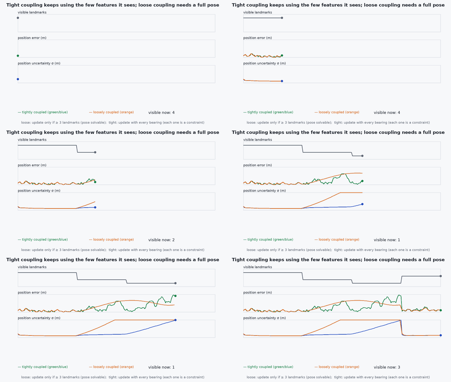
Loosely coupled fusion needs a full camera pose first; tightly coupled fusion can use a single feature: that difference is the reason VIO systems are tightly coupled.
There are two ways to combine a camera and an IMU. Process the images into a pose and fuse that pose, or feed the raw feature observations into the estimator together with the IMU. The second is more complex and extracts more information, particularly when the camera sees little.
Learning objectives
After this lesson, you should be able to:
- Describe loosely and tightly coupled camera-IMU fusion.
- State what information each throws away and when that matters.
- Implement a bearing-only update with one landmark and show its value.
- Explain why time offset and extrinsics belong in the fusion state.
Conceptual explanation
Loosely coupled: a vision module (PnP, VO) produces a pose with covariance; the filter fuses it as a position/orientation measurement. Simple and modular, but a pose needs enough features (at least three points for PnP) and its covariance is an approximation. Tightly coupled: the filter or optimiser receives the raw feature measurements (pixel coordinates), predicts them from the state and uses the residuals directly; features can be used one at a time and their correlations with the state are kept.
Engineering intuition
With only one landmark in view (a doorway after a turn, a few features in a dark room) a vision module cannot compute a pose and returns nothing; the loosely coupled filter then coasts on the IMU. A tightly coupled filter still gets a bearing to that landmark, which constrains the position along a line and, through the correlations with velocity and attitude, improves the whole state. The more often features are scarce, the more tight coupling pays.
Mathematical formulation
A landmark at known (or estimated) world position ℓ is observed as a bearing (ℓ, ℓ) − plus noise. The measurement Jacobian with respect to position and heading is:
The innovation is the wrapped difference between measured and predicted bearing. A single bearing constrains one direction of position and the heading; successive bearings from a moving vehicle constrain the rest (a parallax effect). Observability depends on motion: moving straight toward the landmark gives no new constraint on position across the line of sight.
- bearing to the landmark in the body frame.
- ℓ
- landmark position.
- range to the landmark.
Fusion state augmentation: time offset and camera–IMU extrinsics can be estimated online as additional states (Li and Mourikis; Kelly and Sukhatme), but they must be excited by motion and have a good initial guess (lesson M7-T16).
Architecture and data flow
Feature tracker → pixel measurements with timestamps and covariance → state predicted from the IMU at the image time → measurement residual and Jacobian → filter or optimiser update (lesson M2-T11). VINS-Fusion and OpenVINS are tightly coupled; many PX4 external-vision setups are loosely coupled (the estimator’s pose enters EKF2 as external odometry, lesson M6-T10). Mixing them is fine: a tightly coupled VIO on the companion, its output loosely coupled into EKF2.
Real-world UAV applications
- VIO in feature-poor corridors.
- Landmark-based localisation with fiducial markers.
- Deciding the interface to PX4: external odometry (loose) versus a vision update inside EKF2.
- Online camera–IMU calibration.
Implementation example
This runs as shown: a vehicle moves along a curved path with IMU dead reckoning that drifts. A single known landmark is seen as a bearing; the tightly coupled EKF uses it, while a loosely coupled approach (which needs a pose) gets nothing from one landmark. The bearing update cuts the position error.
import numpy as np
rng = np.random.default_rng(3)
dt, n = 0.1, 600
wrap = lambda a: (a + np.pi) % (2 * np.pi) - np.pi
landmark = np.array([30.0, 15.0])

def truth(t):  # moves on a gentle curve at about 3 m/s
    th = 0.03 * t; v = 3.0
    return np.array([v * np.sin(th) / 0.03, v * (1 - np.cos(th)) / 0.03]), v * np.array([np.cos(th), np.sin(th)]), th

def run(use_bearing):
    x = np.array([0.0, 0.0, 3.0, 0.0, 0.0]); P = np.diag([1, 1, 0.1, 0.1, 0.01]); err = []
    bias = np.array([0.04, -0.03]); Q = np.diag([0, 0, 0.02, 0.02, 1e-5]) * dt; R = np.array([[np.radians(1.0) ** 2]])
    for k in range(n):
        t = k * dt; p, v, th = truth(t)
        a_true = (truth(t + dt)[1] - v) / dt
        a_meas = a_true + bias + 0.05 * rng.standard_normal(2)                       # accelerometer with bias (world frame for simplicity)
        om = 0.03 + 0.003 * rng.standard_normal()
        F = np.eye(5); F[0, 2] = F[1, 3] = dt
        x = np.array([x[0] + x[2] * dt, x[1] + x[3] * dt, x[2] + a_meas[0] * dt, x[3] + a_meas[1] * dt, x[4] + om * dt]); P = F @ P @ F.T + Q
        if use_bearing and k % 5 == 0:
            beta = wrap(np.arctan2(*(landmark - p)[::-1]) - th + np.radians(1.0) * rng.standard_normal())
            d = landmark - x[:2]; rho2 = d @ d
            H = np.array([[d[1] / rho2, -d[0] / rho2, 0, 0, -1.0]])
            y = wrap(beta - (np.arctan2(d[1], d[0]) - x[4])); S = H @ P @ H.T + R; K = (P @ H.T) / S
            x = x + (K * y).ravel(); P = (np.eye(5) - K @ H) @ P @ (np.eye(5) - K @ H).T + K @ R @ K.T
        err.append(np.linalg.norm(x[:2] - p))
    return np.array(err)

e_imu, e_tight = run(False), run(True)
print(f"final position error: IMU only {e_imu[-1]:.1f} m, bearing to one landmark {e_tight[-1]:.1f} m")
assert e_tight[-100:].mean() < 0.5 * e_imu[-100:].mean()Common engineering mistakes
Assuming loosely coupled is always enough
It fails or degrades exactly when features are scarce.
Double use of the same measurements
Feeding VIO output (which already contains the IMU) back with another IMU in a second filter double-counts information.
Ignoring the time offset
Both the pose and the feature residuals shift (lesson M7-T8).
Fusing pose with an overconfident covariance
Loose coupling is only as good as the vision covariance.
No excitation for online calibration
Extrinsics and time offset are unobservable without motion.
Failure modes
| Failure mode | How it shows up | Likely cause |
|---|---|---|
| Dropout of vision pose | Filter coasts | Too few features for a pose in a loosely coupled design |
| Inconsistency | Over-confident output | Double counting or ignored correlations |
| Extrinsic drift | Slow rotation-dependent error | Wrong extrinsics or time offset |
| Observability loss in straight flight | Cross-line-of-sight uncertainty grows | No parallax from motion |
Debugging approach
- Compare filter output with vision-only and IMU-only references.
- Plot the number of features per frame and estimator covariance.
- Check residual statistics per feature track.
- Vary the time offset and see the residuals.
Practical exercises
- Use two landmarks and compare the position error with one.
- Show that moving straight toward the landmark leaves the cross-range uncertainty unchanged.
- Add the time offset as a state and estimate it.
- Decide for your design whether the PX4 interface should be loose or tight.
Interview questions
Write an answer in your own words, then reveal the model answer. Nothing is sent anywhere.
Question 1
What is the difference between loosely and tightly coupled fusion?
Model answer
Loose: fuse a pose produced by a vision module; tight: feed raw feature observations and IMU into one estimator, retaining correlations and using even single features.
Question 2
When does tight coupling pay most?
Model answer
When features are scarce or intermittent, because a pose cannot be computed but individual measurements still constrain the state.
Question 3
Why must the time offset be considered?
Model answer
The images and IMU samples refer to different instants if the offset is wrong, which biases the residuals especially in fast motion.
References and further reading
Primary papers, official documentation and standards. Each claim above that is specific to a tool or version points here.