UAV Systems Engineering · Module 3
M3-T8: IMU preintegration
Integrate the IMU once between keyframes into a relative-motion measurement, so the optimiser can change its mind without re-integrating hundreds of samples.
Every tightly coupled VIO and LIO system faces the same problem: the IMU runs at hundreds of hertz, the optimisation at tens, and the states keep changing as the solver iterates. Preintegration (Lupton and Sukkarieh; Forster et al.) is the answer, and its core is a few lines of code you can check against direct integration.
Learning objectives
After this lesson, you should be able to:
- Define the preintegrated measurements , and and why they do not depend on the world pose.
- Reconstruct the state at keyframe from the state at and the preintegrated terms.
- Explain first-order bias correction and why re-integration is avoided.
- Verify preintegration numerically against direct propagation.
Conceptual explanation
Directly propagating the IMU from keyframe to requires the full state and every sample; if the optimiser later changes or , the integration must be redone. Preintegration rewrites the integral in the body frame of keyframe so that it depends only on the IMU samples and the biases, not on the world state at . The estimator then treats the three increments as one measurement linking the two keyframes.
Engineering intuition
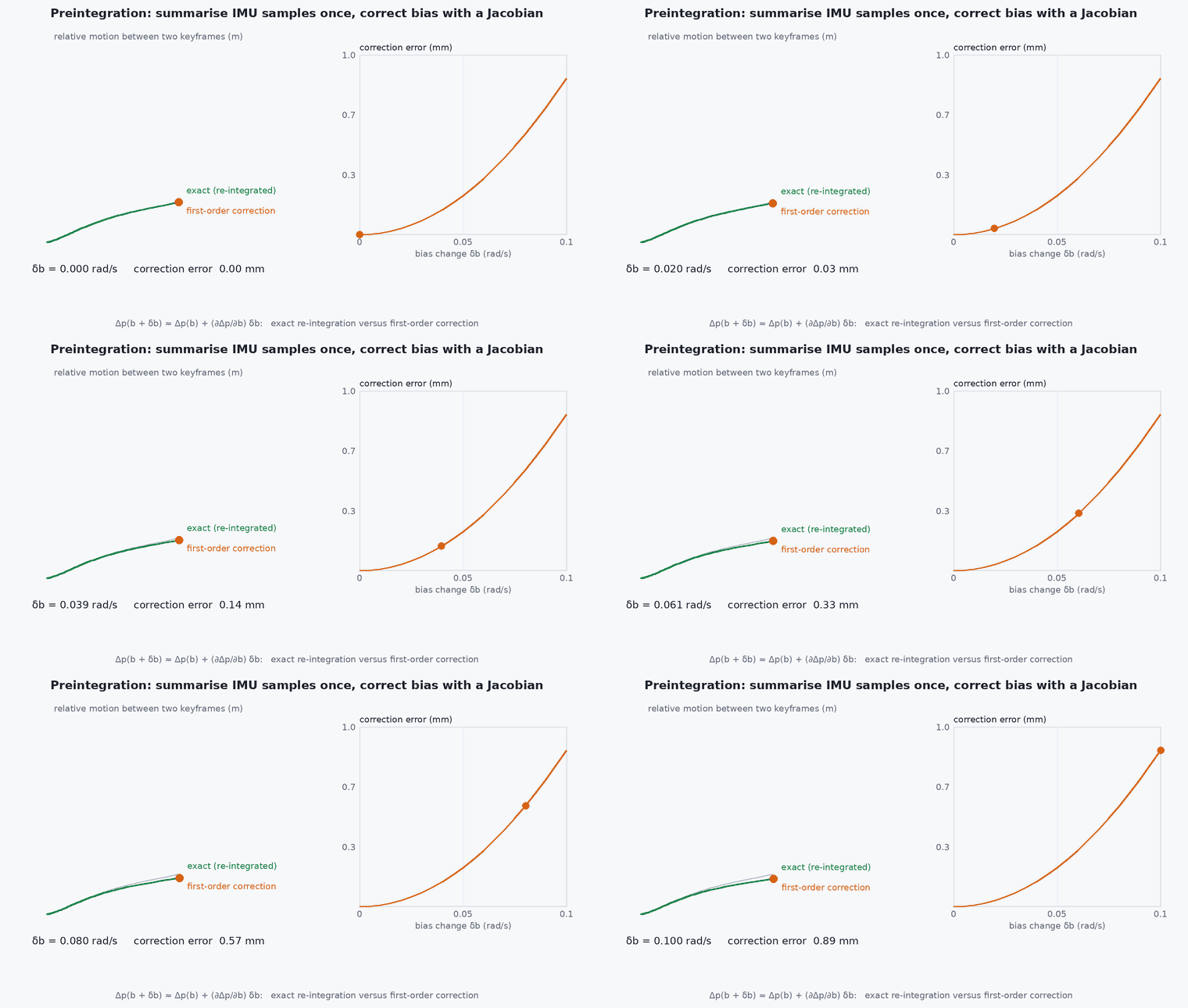
Gravity and the unknown initial velocity are what tie a naive integration to the world state. Preintegration removes them from the integral: it integrates only the body-frame measured rotation and specific force relative to the start, and adds gravity and initial velocity analytically afterwards. The increments are therefore reusable. The remaining dependency is the bias, which changes slowly: instead of re-integrating, a first-order (Jacobian) correction updates the increments for a small bias change.
Mathematical formulation
With samples at interval , biases and the rotation accumulated since keyframe :
The state at keyframe follows from the state at , the time and gravity (world frame):
This is exactly what direct integration produces (for the same discretisation), which is the test below. A noise model propagates the IMU noise densities through the recursion into a 9×9 covariance of , which weights the factor in the optimisation. For small bias changes , the increments are updated by first-order Jacobians accumulated during preintegration, avoiding re-integration:
Forster et al. (2017) give the manifold-consistent derivation, including the covariance recursion and the Jacobians; use that paper when implementing a real system.
Architecture and data flow
IMU samples between two camera or LiDAR timestamps → preintegrator (accumulates , , , Jacobians and covariance) → factor between keyframes and (and the bias random-walk factor) → sliding-window optimiser or smoother (VINS-Fusion, OpenVINS-style filters use related ideas). IMU samples must be interpolated exactly at the keyframe timestamps, which is why the camera-IMU time offset (lesson M7-T8) is part of the estimation: a time error shifts where the integration begins and ends.
Real-world UAV applications
- VINS-Fusion and similar sliding-window estimators.
- Factor-graph smoothing in GTSAM-based VIO.
- LiDAR-inertial systems that need the motion between scans.
- Fast re-linearisation in optimisation: the Jacobians avoid re-integration at every iteration.
Implementation example
This runs as shown: it propagates a state for one second directly, then reconstructs the same final state from the preintegrated increments, with a rotating body and non-zero biases. It also shows the first-order bias correction reproducing re-integration to about 1e-7.
import numpy as np
hat = lambda w: np.array([[0, -w[2], w[1]], [w[2], 0, -w[0]], [-w[1], w[0], 0]])
def expm(w):
    th = np.linalg.norm(w)
    if th < 1e-12: return np.eye(3) + hat(w)
    K = hat(w / th); return np.eye(3) + np.sin(th) * K + (1 - np.cos(th)) * K @ K
def logm(R):
    th = np.arccos(np.clip((np.trace(R) - 1) / 2, -1, 1))
    return np.zeros(3) if th < 1e-9 else th / (2 * np.sin(th)) * np.array([R[2, 1] - R[1, 2], R[0, 2] - R[2, 0], R[1, 0] - R[0, 1]])

g = np.array([0, 0, -9.81]); dt, n = 0.005, 200; T = n * dt
gyro = np.array([[0.5 * np.sin(0.02 * k) + 0.1, 0.3 * np.cos(0.03 * k), 0.4] for k in range(n)])          # measured rate (rad/s)
acc = np.array([[1 + np.sin(0.05 * k), 0.5 * np.cos(0.04 * k), 9.81 + 0.3 * np.sin(0.07 * k)] for k in range(n)])   # measured specific force
bg, ba = np.array([0.01, -0.02, 0.015]), np.array([0.05, 0.02, -0.03])
R0, v0, p0 = expm(np.array([0.2, -0.1, 0.5])), np.array([1.0, 0.5, 0.0]), np.array([0.0, 0.0, 1.0])

# direct propagation in the world frame
R, v, p = R0.copy(), v0.copy(), p0.copy()
for k in range(n):
    a = R @ (acc[k] - ba) + g
    p = p + v * dt + 0.5 * a * dt * dt; v = v + a * dt; R = R @ expm((gyro[k] - bg) * dt)

def preintegrate(bg_, ba_):                                      # body-frame increments: independent of R0, v0, p0 and gravity
    dR, dv, dp = np.eye(3), np.zeros(3), np.zeros(3)
    for k in range(n):
        a = acc[k] - ba_
        dp = dp + dv * dt + 0.5 * dR @ a * dt * dt; dv = dv + dR @ a * dt; dR = dR @ expm((gyro[k] - bg_) * dt)
    return dR, dv, dp
dR, dv, dp = preintegrate(bg, ba)
R_j, v_j, p_j = R0 @ dR, v0 + g * T + R0 @ dv, p0 + v0 * T + 0.5 * g * T * T + R0 @ dp
print("max reconstruction error  R: %.1e  v: %.1e  p: %.1e" % (np.abs(R_j - R).max(), np.abs(v_j - v).max(), np.abs(p_j - p).max()))
assert np.abs(R_j - R).max() < 1e-12 and np.abs(v_j - v).max() < 1e-10 and np.abs(p_j - p).max() < 1e-10

# first-order bias correction of the rotation increment
dbg = np.array([0.002, 0.001, -0.001]); dR0 = dR; dR1 = preintegrate(bg + dbg, ba)[0]
J = np.column_stack([logm(dR0.T @ preintegrate(bg + e, ba)[0]) / 1e-6 for e in 1e-6 * np.eye(3)])   # numerical d(log dR)/d(bg)
err_corrected = np.abs(dR0 @ expm(J @ dbg) - dR1).max(); err_none = np.abs(dR0 - dR1).max()
print(f"bias change: error without correction {err_none:.1e}, with first-order Jacobian {err_corrected:.1e}")
assert err_corrected < err_none / 1000Common engineering mistakes
Integrating in the world frame
Then the result depends on the current estimate of and must be redone at every optimiser iteration.
Forgetting gravity and the initial velocity in the reconstruction
They are added back analytically; omitting them gives a vehicle that floats.
Re-integrating on every bias update
Use the first-order Jacobian correction for small changes and re-integrate only when the bias moves a lot.
Interpolating IMU data at wrong timestamps
Keyframe times must align with the IMU stream, including the camera-IMU offset.
Inconsistent covariance
Wrong noise densities (lesson M3-T7) mis-weight the factor and the filter becomes overconfident or sluggish.
Failure modes
| Failure mode | How it shows up | Likely cause |
|---|---|---|
| Drift with a stationary vehicle | Slow motion estimate at rest | Bias not estimated or noise parameters wrong |
| Scale error in visual-inertial odometry | Trajectory size wrong | IMU excitation too low to observe scale, or gravity direction not initialised |
| Divergence after fast rotation | Estimate explodes after aggressive yaw | Gyro saturation or time offset; first-order bias correction invalid for large changes |
| Wrong gravity magnitude | Constant climb or sink in the estimate | Gravity constant or direction wrong in the initialisation |
Debugging approach
- Test the preintegrator against direct integration on synthetic data, as above.
- Check the covariance by Monte Carlo: simulate many noisy samples and compare the sample covariance of the increments.
- Plot estimated biases over the flight; they should be smooth and within the sensor’s specification.
- Vary the camera-IMU time offset and watch the residuals.
Practical exercises
- Show that , and are unchanged if , and change (modify the code).
- Measure the error of the first-order correction as a function of the size of .
- Add white noise to the samples and estimate the covariance of by Monte Carlo.
- Compute the number of IMU samples saved per keyframe for a 200 Hz IMU and a 20 Hz camera.
Interview questions
Write an answer in your own words, then reveal the model answer. Nothing is sent anywhere.
Question 1
Why is preintegration useful in a sliding-window estimator?
Model answer
The relative-motion increments do not depend on the world pose and velocity at the start, so the optimiser can change those states without re-integrating hundreds of IMU samples; bias changes are handled with first-order Jacobians.
Question 2
What has to be added back when reconstructing the state from the increments?
Model answer
The initial velocity and gravity over the interval, and the initial rotation to express the body-frame increments in the world frame.
Question 3
Which IMU error terms does preintegration carry?
Model answer
Bias (corrected to first order via Jacobians) and white noise (propagated into a covariance), plus the bias random walk as a separate factor between keyframes.
References and further reading
Primary papers, official documentation and standards. Each claim above that is specific to a tool or version points here.
- C. Forster, L. Carlone, F. Dellaert, D. Scaramuzza, “On-manifold preintegration for real-time visual-inertial odometry”, IEEE T-RO, 2017
- Forster et al. on arXiv:1512.02363
- T. Lupton, S. Sukkarieh, “Visual-inertial-aided navigation for high-dynamic motion in built environments without initial conditions”, IEEE T-RO, 2012
- T. Qin, P. Li, S. Shen, “VINS-Mono”, arXiv:1708.03852