UAV Systems Engineering · Module 3
M3-T10: LiDAR-IMU fusion
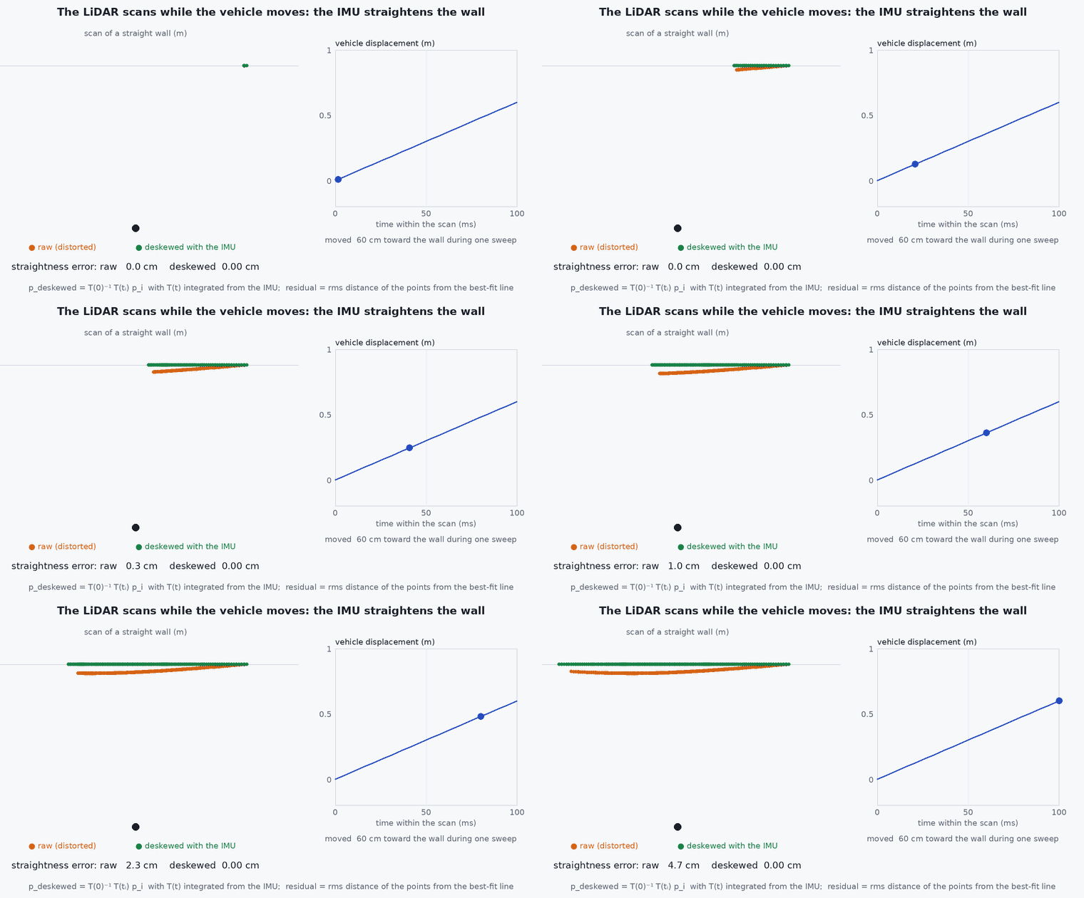
A LiDAR scan is not a snapshot: it takes a tenth of a second while the vehicle moves, and the IMU is what lets you put every point on one instant.
At UAV speeds a rotating or scanning LiDAR distorts its own scan. LiDAR-IMU fusion removes the distortion with the IMU’s motion estimate, and then uses the scan to correct the IMU’s drift. This lesson builds the deskewing step and the structure of the filter around it.
Learning objectives
After this lesson, you should be able to:
- Explain motion distortion of a scan and how IMU motion removes it.
- Describe the structure of a tightly coupled LiDAR-inertial filter (propagate, deskew, register, update).
- Compute the size of the distortion for a given speed and rotation rate.
- State the roles of the LiDAR-IMU extrinsics and time offset.
Conceptual explanation
A LiDAR measures points sequentially over the scan period (typically 0.05–0.1 s). Each point is measured in the sensor frame at its own time, while the sensor moves. If the points are simply stacked, straight walls bend. Deskewing expresses every point in the sensor frame at one reference time (the scan end) using the sensor’s motion during the scan, interpolated from the IMU.
Engineering intuition
At 10 m/s and a 0.1 s scan the vehicle moves one metre during a scan; a yaw rate of 60°/s turns the sensor by , which at 20 m range displaces points by over two metres. Ignoring that smears the map and the registration residuals. The IMU, at hundreds of hertz, tells precisely how the sensor moved within the scan: integrating it gives a pose for each point’s timestamp. The LiDAR in turn corrects the IMU’s accumulated errors every scan: each sensor repairs the other’s weakness.
Mathematical formulation
With the IMU-propagated sensor pose and the reference time , a point measured at time in the sensor frame is expressed in the end-of-scan frame by:
With constant velocity and angular rate over the scan: and . The un-corrected displacement of a point at range is roughly , maximal for the first point of the scan. The measurement model is then the point-to-plane residual of lesson M2-T13 in the end-of-scan frame, and the state update is an iterated Kalman update (lesson M4-T8).
- ,
- timestamp of a point and of the scan end.
- ,
- IMU-propagated rotation and position at those times.
- scan duration.
The LiDAR–IMU extrinsics enter every transformation above; an error of in displaces points at 20 m by 0.35 m. The time offset between the clocks acts like a motion error: rotation, translation (lesson M7-T8).
Architecture and data flow
Requirements: per-point timestamps in the point-cloud message, a calibrated extrinsic transform, a shared or synchronised clock, and an IMU at 100 Hz or more. Output: odometry and covariance, undistorted registered cloud, map. Feed the odometry to PX4 as external vision after frame and timestamp handling (lesson M6-T10).
Real-world UAV applications
- LiDAR-inertial odometry for fast UAVs (Capstone 2).
- Mapping with a handheld or aerial LiDAR.
- Obstacle maps with correct geometry at speed.
- Tight coupling with vision (FAST-LIVO2, lesson M4-T10).
Implementation example
This runs as shown: a wall scanned while the sensor translates and yaws is distorted; deskewing with the (exact) motion removes the distortion, and a 10 ms time-offset error brings back part of it.
import numpy as np
T_scan, n = 0.1, 400
v = np.array([8.0, 0.0]); om = np.radians(60.0)                    # 8 m/s forward, 60 deg/s yaw during the scan
R2 = lambda a: np.array([[np.cos(a), -np.sin(a)], [np.sin(a), np.cos(a)]])

def pose(t):                                                       # sensor pose in the world at time t (scan starts at t = 0)
    return R2(om * t), v * t
walls_y = 6.0                                                      # a straight wall y = 6 m (world frame)
times = np.linspace(0, T_scan, n); pts_sensor = []
for t in times:                                                    # beam direction sweeps 180 degrees over the scan; the sensor moves while it does
    R, p = pose(t); a = np.pi * t / T_scan
    d = R @ np.array([np.cos(a), np.sin(a)])
    if d[1] > 0.2: pts_sensor.append((t, np.array([np.cos(a), np.sin(a)]) * (walls_y - p[1]) / d[1]))   # range to the wall along the beam
t_pts = np.array([t for t, _ in pts_sensor]); P = np.array([p for _, p in pts_sensor])

def to_end_frame(t_i, P_i, dt_err=0.0):                             # deskew: sensor frame at t_i -> sensor frame at the scan end
    Re, pe = pose(T_scan); out = []
    for t, p in zip(t_i, P_i):
        R, pp = pose(t + dt_err); out.append(Re.T @ (R @ p + pp - pe))
    return np.array(out)

def wall_flatness(Q):                                              # transform back to the world with the end pose and measure the spread across the wall
    Re, pe = pose(T_scan); W = (Q @ Re.T) + pe; return W[:, 1].std()

raw = (P @ pose(T_scan)[0].T) + pose(T_scan)[1]                    # stacking points without deskewing (as if all taken at the end pose)
print(f"wall thickness (std of y): raw {raw[:, 1].std():.3f} m, deskewed {wall_flatness(to_end_frame(t_pts, P)):.4f} m, deskewed with 10 ms offset {wall_flatness(to_end_frame(t_pts, P, 0.01)):.3f} m")
assert wall_flatness(to_end_frame(t_pts, P)) < 1e-9 and raw[:, 1].std() > 0.5
assert 1e-9 < wall_flatness(to_end_frame(t_pts, P, 0.01)) < raw[:, 1].std() / 3Common engineering mistakes
Skipping deskewing because scans look fine when slow
The distortion scales with speed and rotation rate; manoeuvres expose it.
Using message arrival time for points
Per-point or per-packet LiDAR time is required.
Wrong extrinsic rotation
Systematic map smear that rotates with the vehicle.
Constant-velocity deskewing during hard manoeuvres
Use the IMU samples within the scan, not a single average.
Ignoring the LiDAR blind zone and airframe returns
Filter points on the vehicle.
Failure modes
| Failure mode | How it shows up | Likely cause |
|---|---|---|
| Double walls in the map | Smeared structures in turns | Time offset or extrinsic error |
| Registration failure at speed | Odometry jumps in fast manoeuvres | No deskewing or IMU saturation |
| Vibration blur | Fuzzy surfaces in hover | IMU noise or motor vibration |
| Drift in corridors | Along-axis drift | Degenerate geometry (lesson M2-T13) |
Debugging approach
- Fly a rotation in place and look at the accumulated cloud for ghosting.
- Check per-point timestamps for monotonic order and correct units.
- Compare cloud thickness of a known flat wall with and without deskewing.
- Estimate the time offset using the IMU–LiDAR rotation correlation (lesson M7-T8).
Practical exercises
- Compute the distortion at 20 m for 30°/s over a 0.1 s scan.
- Run the example with a 20°/s yaw rate and plot the thickness against rate.
- Estimate the extrinsic rotation error that gives 0.1 m displacement at 30 m.
- Describe what to log to check LiDAR-IMU synchronisation.
Interview questions
Write an answer in your own words, then reveal the model answer. Nothing is sent anywhere.
Question 1
What is motion distortion and how is it corrected?
Model answer
Points in one scan are measured at different times while the sensor moves; each point is transformed to a common reference time using the IMU-propagated pose at its timestamp.
Question 2
Why do LiDAR and IMU complement each other?
Model answer
The IMU provides high-rate motion for deskewing and prediction but drifts; LiDAR registration corrects the drift and biases each scan.
Question 3
Which calibration terms enter LiDAR-IMU fusion?
Model answer
The rotation and translation between the sensors and the time offset between their clocks.
References and further reading
Primary papers, official documentation and standards. Each claim above that is specific to a tool or version points here.