UAV Systems Engineering · Module 7
M7-T16: Camera-IMU-LiDAR extrinsic calibration
Extrinsics are the unglamorous numbers that make fusion work. Estimate them with rich motion, and verify them against something you did not fit.
A camera and an IMU on one vehicle see the same motion through different frames and clocks. The extrinsic calibration is the fixed rotation and translation between their frames, and the time offset between their clocks. Errors here produce drift and instability in VIO that no filter tuning will remove.
Learning objectives
After this lesson, you should be able to:
- Define the extrinsic parameters and the time offset and state what excitation observes each.
- Estimate rotation by aligning angular-rate vectors and the time offset by correlating rate magnitudes.
- Explain why translation is weakly observable and what motion improves it.
- Design an independent validation for the calibrated result.
Conceptual explanation
Established The formulations follow standard practice (angular-rate alignment, Kalibr-style continuous-time calibration, LiDAR-IMU calibration methods). Achievable accuracy depends on the sensors, the excitation and the target; none is claimed here.
The parameters:
- Rotation between the camera and IMU frames: observable from any rotation, since the angular velocity of one rigid body expressed in two frames differs by exactly .
- Translation (the lever arm): observable only when the body accelerates, because the rotation-induced acceleration at the camera, , is what depends on it. Small lever arms (a few centimetres) need strong rotational acceleration to be resolved.
- Time offset : observable from the time shift that best aligns the two sensors’ motion signals, again requiring rotation (a static or slow trajectory has no signal to align).
- LiDAR-IMU: similar structure, but the “camera” measurement is a registration of point clouds; the same excitation requirements apply, and the scan-time distortion of spinning LiDARs must be modelled.
Engineering intuition
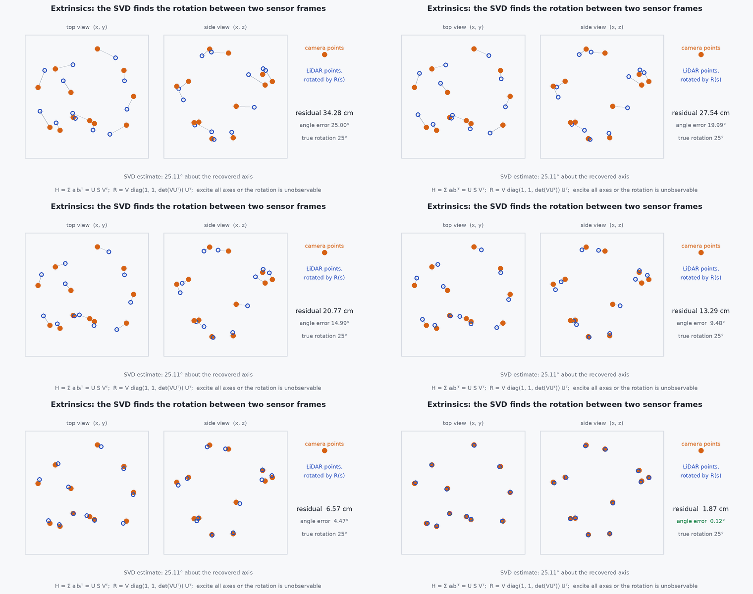
If you spin the vehicle, both the gyro and the camera (through visual odometry) report the same angular velocity vector, but in different coordinates. The rotation that maps one set of vectors onto the other is the extrinsic rotation: a 3D point-alignment problem, solved exactly by the SVD (Kabsch/Arun method). The time offset is the shift that makes the two angular-rate signals overlap.
The translation is a harder and more fragile measurement: it depends on accelerations that the IMU measures with noise, and it correlates with the accelerometer bias and gravity direction. Expect a few millimetres to a centimetre of uncertainty even with good excitation, and do not trust a translation estimated from a smooth, slow trajectory.
Mathematical formulation
The angular velocities in the two frames are related by , up to noise (the sign convention of must be fixed and documented). For time-aligned samples, the rotation minimising is found by SVD of the cross-covariance:
The time offset maximises the correlation of the rate magnitudes (which does not depend on the unknown rotation): after resampling to a common grid; refine to a fraction of the sample period by interpolating the correlation peak. A necessary condition for observability of the rotation is that the angular velocity vectors span three dimensions: the matrix must have rank 3, in practice a well-conditioned smallest singular value. Translation enters through the specific-force difference:
- ,
- rotation and translation between camera and IMU frames.
- time offset between the sensors.
- , , ,
- cross-covariance and its SVD.
Architecture and data flow
Recorded rosbag of the excitation motion (IMU at hundreds of Hz, camera at 20–30 Hz with its stamps) → calibration tool (Kalibr for camera-IMU with a target, or a LiDAR-IMU tool) → extrinsics file (, , d, covariance) → the VIO or LiDAR-inertial pipeline’s configuration. The same file is used by the TF publisher. The tool’s covariance output and the validation residuals are stored with it.
Real-world UAV applications
- Setting up VIO before the first flight.
- Checking a camera mount after a repair.
- Calibrating LiDAR-IMU for LiDAR-inertial odometry.
- Diagnosing why a VIO that works on one vehicle fails on another of the same type.
Implementation example
This runs as shown. Synthetic angular-rate data for a rotating vehicle: an IMU at 200 Hz and a visual-odometry angular rate at 30 Hz, with a 37 ms time offset and a fixed rotation. The code estimates the offset by correlating rate magnitudes, then the rotation by the SVD, and validates on a second, independent motion.
import numpy as np
rng = np.random.default_rng(14)
def rotvec(w):
    th = np.linalg.norm(w); K = np.array([[0, -w[2], w[1]], [w[2], 0, -w[0]], [-w[1], w[0], 0]]) / (th if th > 0 else 1)
    return np.eye(3) + np.sin(th) * K + (1 - np.cos(th)) * K @ K
R_true = rotvec(np.array([0.3, -0.5, 1.9])); t_d_true = 0.037               # camera-to-IMU rotation, and the delay of the camera stamps

def omega(t, seed):                                                         # smooth rich angular velocity: sums of sinusoids with different frequencies per axis
    r = np.random.default_rng(seed); f = r.uniform(0.3, 1.5, (3, 3)); p = r.uniform(0, 6.28, (3, 3)); a = r.uniform(0.4, 1.2, (3, 3))
    return sum(a[:, i:i + 1] * np.sin(2 * np.pi * f[:, i:i + 1] * t + p[:, i:i + 1]) for i in range(3)).T
def make(seed, T=30.0):
    t_i = np.arange(0, T, 1 / 200.0); w_i = omega(t_i, seed) + 0.01 * rng.standard_normal((t_i.size, 3))        # IMU gyro
    t_c = np.arange(1.0, T - 1.0, 1 / 30.0)
    w_c = (omega(t_c - t_d_true, seed) @ R_true) + 0.02 * rng.standard_normal((t_c.size, 3))                    # VO angular rate in the camera frame (camera stamps lag by t_d)
    return t_i, w_i, t_c, w_c
def estimate_td(t_i, w_i, t_c, w_c, span=0.1, step=0.0005):
    n_i = np.linalg.norm(w_i, axis=1); n_c = np.linalg.norm(w_c, axis=1); best = None
    for tau in np.arange(-span, span, step):                                # shift the camera stamps by tau and compare magnitudes on the camera grid
        m = np.interp(t_c - tau, t_i, n_i); c = np.corrcoef(m, n_c)[0, 1]
        if best is None or c > best[0]: best = (c, tau)
    return best[1]
def estimate_R(t_i, w_i, t_c, w_c, td):
    wi = np.stack([np.interp(t_c - td, t_i, w_i[:, a]) for a in range(3)], axis=1)
    H = w_c.T @ wi; U, S, Vt = np.linalg.svd(H); D = np.diag([1, 1, np.linalg.det(Vt.T @ U.T)])
    return Vt.T @ D @ U.T, S
d1 = make(1); td = estimate_td(*d1); R, S = estimate_R(*d1, td)
ang = lambda A, B: np.degrees(np.arccos(np.clip((np.trace(A.T @ B) - 1) / 2, -1, 1)))
print(f"time offset estimate {td * 1e3:.1f} ms (true {t_d_true * 1e3:.1f}); rotation error {ang(R, R_true):.3f} deg; singular values {np.round(S, 1)}")
d2 = make(2)                                                                 # independent validation motion, not used for fitting
wi2 = np.stack([np.interp(d2[2] - td, d2[0], d2[1][:, a]) for a in range(3)], axis=1)
res = np.sqrt(np.mean(np.linalg.norm(wi2 - d2[3] @ R.T, axis=1) ** 2)); res0 = np.sqrt(np.mean(np.linalg.norm(wi2 - d2[3], axis=1) ** 2))
print(f"validation residual of angular rates: calibrated {res:.3f} rad/s, uncalibrated {res0:.3f} rad/s")
assert abs(td - t_d_true) < 0.003 and ang(R, R_true) < 0.5 and res < 0.05 and res0 > 5 * res and S[2] > 0.1 * S[0]Common engineering mistakes
Calibrating with a slow or planar motion
Rotation about one axis leaves the others unobservable; excite all three axes.
Estimating translation from gentle motion
It needs rotational acceleration; expect a large uncertainty otherwise.
Fitting and validating on the same data
Validate on a separate motion or against an external reference (a motion-capture trajectory).
Ignoring the time offset
A few milliseconds of offset looks like a rotation error during fast turns.
Sign convention confusion
Define extrinsics as or and the offset sign in the file; apply consistently.
Failure modes
| Failure mode | How it shows up | Likely cause |
|---|---|---|
| VIO scale drift | Bias in position estimates | Wrong translation or time offset |
| Divergence in fast rotations | Tracking loss at high angular rates | Time offset or rotation error |
| Calibration differs between runs | Parameters do not repeat | Insufficient excitation; poorly observable parameters |
| Good fit but poor flight | Residuals are small, flight bad | Over-fitting to a motion not representative of flight |
Debugging approach
- Plot the angular-rate signals before and after alignment.
- Check the singular values of the cross-covariance: a small third value means poor excitation.
- Repeat the calibration on separate recordings and compare the spread.
- Test the result in VIO with an external reference trajectory.
Practical exercises
- Reduce the motion to rotation about one axis in the example and report the singular values and the rotation error.
- Compute the acceleration signal at a 5 cm lever arm for and ; compare with accelerometer noise of .
- Add a gyro bias of 0.02 rad/s and see how it affects the rotation estimate.
- Design the validation procedure for the extrinsics of your vehicle.
Interview questions
Write an answer in your own words, then reveal the model answer. Nothing is sent anywhere.
Question 1
What excitation is needed to calibrate camera-IMU extrinsics?
Model answer
Rotation about all three axes for the rotation and time offset, and rotational acceleration (plus translation) for the lever arm; slow or planar motion leaves parameters unobservable.
Question 2
How can you estimate the time offset without knowing the rotation?
Model answer
Correlate the magnitudes of the angular rates of the two sensors, which are independent of the rotation between the frames, and find the shift that maximises the correlation.
Question 3
Why is validation on separate data necessary?
Model answer
A calibration can fit its own motion well while being wrong for others (over-fitting or low observability); independent data or an external reference reveals this.
References and further reading
Primary papers, official documentation and standards. Each claim above that is specific to a tool or version points here.
- Arun, K. S., Huang, T. S. & Blostein, S. D. (1987). Least-squares fitting of two 3-D point sets. IEEE TPAMI 9(5)
- Furgale, P., Rehder, J. & Siegwart, R. (2013). Unified temporal and spatial calibration for multi-sensor systems. IROS
- Kalibr wiki: multi-camera and camera-IMU calibration
- LiDAR_IMU_Init: LiDAR-IMU initialisation and calibration