UAV Systems Engineering · Module 3
M3-T6: Error-State Kalman Filter
Keep the big nonlinear state outside the filter and estimate only its small error: that keeps rotations on the manifold and the linearisation honest.
Autopilots such as PX4’s EKF2 are error-state filters. The reason is rotation: a three-parameter error stays small and well-behaved even when the attitude itself is arbitrary. This lesson builds a complete attitude ESKF in thirty lines.
Learning objectives
After this lesson, you should be able to:
- Explain the nominal, error and true states and the injection and reset steps.
- Write the attitude error-state propagation and gravity measurement update.
- Run an ESKF that estimates attitude and gyro bias, and check it against truth.
- State what remains unobservable (yaw from gravity alone).
Conceptual explanation
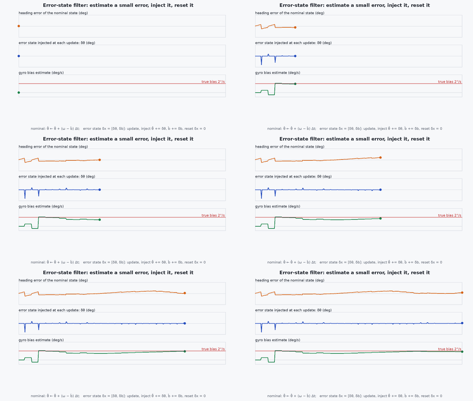
An error-state (indirect) filter splits the state into a nominal state propagated with the full nonlinear equations and an error state , small, Gaussian and estimated by a linear filter. Measurements update ; the estimate is then injected into the nominal state and is reset to zero (with a small covariance correction).
Engineering intuition
The nominal rotation can be anything; the error between estimate and truth is small if the filter works, so its first-order (small-angle) model is accurate where it matters, around zero. A quaternion or rotation matrix in the state would need a constraint (unit norm) that a linear Kalman update does not respect; a three-component error rotation vector has none. Zero is also where the error-state dynamics are best conditioned, and where they cost least to linearise.
Mathematical formulation
Attitude (body to world) with true (error in the body frame), gyro bias error and measured rate :
A gravity-direction measurement (accelerometer with negligible linear acceleration), + noise, predicted as . To first order the innovation is ₓ , so = [ []ₓ 0 ]. Standard Kalman update gives ; then:
Gravity measures only roll and pitch: the rotation about the vertical (yaw) is unobservable from it, so yaw drifts at the unestimated part of the gyro bias until a magnetometer, vision or GNSS heading supplies it (lessons M3-T12 and M2-T11). The same structure extends to position, velocity and accelerometer bias for the full navigation filter (Solà 2017).
- attitude error as a rotation vector (small).
- gyro bias error.
- [·]ₓ
- skew-symmetric (cross-product) matrix.
- Exp
- exponential map from rotation vector to rotation matrix.
Architecture and data flow
PX4’s EKF2 follows this pattern for full navigation: it propagates a nominal state with delayed-horizon IMU data and estimates error states with GNSS, barometer, magnetometer and external-vision updates, with innovation gates (lesson M6-T5). The accelerometer correction of roll and pitch comes via the velocity and position measurements rather than a gravity vector, since the vehicle accelerates.
Real-world UAV applications
- Attitude estimation on every autopilot.
- The core of visual-inertial and LiDAR-inertial filters (OpenVINS, FAST-LIO2).
- Estimating gyro bias in flight.
- Any estimator with rotations in its state.
Implementation example
This runs as shown: an attitude ESKF with gravity updates tracks a rotating body with a gyro bias, keeping tilt error below half a degree and estimating the bias, whereas pure gyro integration drifts by tens of degrees.
import numpy as np
hat = lambda w: np.array([[0, -w[2], w[1]], [w[2], 0, -w[0]], [-w[1], w[0], 0]])
def expm(w):
    th = np.linalg.norm(w)
    if th < 1e-12: return np.eye(3) + hat(w)
    K = hat(w / th); return np.eye(3) + np.sin(th) * K + (1 - np.cos(th)) * K @ K

def run(use_update, seed=0, n=6000, dt=0.01):
    rng = np.random.default_rng(seed); g, sg, sa = 9.81, 0.002, 0.05
    bg_true = np.array([0.02, -0.01, 0.015]); z_up = np.array([0, 0, 1.0])
    Rt = np.eye(3); Rh = expm(np.array([0.2, -0.15, 0.0])); bh = np.zeros(3)         # initial attitude error: 0.25 rad = 14 degrees
    P = np.diag([0.3**2] * 3 + [0.05**2] * 3); Q = np.diag([sg**2 * dt] * 3 + [(1e-5) ** 2 * dt] * 3); Rm = np.eye(3) * (sa / g) ** 2
    tilt = []
    for k in range(n):
        w = np.array([0.3 * np.sin(0.01 * k), 0.2 * np.cos(0.013 * k), 0.1]); Rt = Rt @ expm(w * dt)
        gm = w + bg_true + sg / np.sqrt(dt) * rng.standard_normal(3)
        Rh = Rh @ expm((gm - bh) * dt)                                                # nominal propagation (nonlinear)
        F = np.eye(6); F[:3, :3] = expm(-(gm - bh) * dt); F[:3, 3:] = -np.eye(3) * dt; P = F @ P @ F.T + Q   # error-state covariance propagation
        if use_update and k % 5 == 0:
            z = Rt.T @ z_up + (sa / g) * rng.standard_normal(3); h = Rh.T @ z_up       # gravity direction measured vs predicted
            H = np.zeros((3, 6)); H[:, :3] = hat(h)
            K = P @ H.T @ np.linalg.inv(H @ P @ H.T + Rm); dx = K @ (z - h)
            Rh = Rh @ expm(dx[:3]); bh = bh + dx[3:]                                  # inject, then reset the error state
            IKH = np.eye(6) - K @ H; P = IKH @ P @ IKH.T + K @ Rm @ K.T
        tilt.append(np.degrees(np.arccos(np.clip((Rt.T @ z_up) @ (Rh.T @ z_up), -1, 1))))
    return np.array(tilt), bh, bg_true

tilt_f, bh, bg = run(True); tilt_g, _, _ = run(False)
print(f"tilt error: filter max after 10 s {tilt_f[1000:].max():.2f} deg, gyro-only at the end {tilt_g[-1]:.1f} deg; bias estimate {np.round(bh, 4)} vs {bg}")
assert tilt_f[1000:].max() < 0.5 and tilt_g[-1] > 10
assert np.all(np.abs(bh - bg) < 0.005)Common engineering mistakes
Linear accelerometer-gravity update while accelerating
The gravity assumption fails in manoeuvres; gate it or use velocity aiding.
Forgetting the reset Jacobian
Small but real covariance error for large corrections.
Mixing error conventions (body versus world)
The sign and frame of must match the and matrices.
Estimating yaw from gravity
Not observable: it needs another heading source.
Non-symmetric P
Use the Joseph form.
Failure modes
| Failure mode | How it shows up | Likely cause |
|---|---|---|
| Tilt error during aggressive manoeuvres | Attitude wanders when accelerating | Gravity update trusted despite linear acceleration |
| Yaw drift | Heading slowly rotates | No heading source |
| Bias not converging | Persistent drift | Insufficient rotation excitation or too small |
| Divergence after a large initial error | Filter fails to converge | Initial error beyond the linearisation region |
Debugging approach
- Compare against truth on synthetic data as above.
- Plot bias estimates and covariance.
- Check innovations of the gravity update against their expected variance.
- Test with injected linear accelerations.
Practical exercises
- Add position and velocity states with accelerometer bias and GNSS updates.
- Show numerically that yaw error grows while tilt stays bounded.
- Remove the reset Jacobian and compare covariance consistency.
- Replace the rotation matrix by a quaternion nominal state.
Interview questions
Write an answer in your own words, then reveal the model answer. Nothing is sent anywhere.
Question 1
Why use an error-state filter for attitude?
Model answer
The error is a small three-vector that needs no constraint and is well approximated by a linear model, while the nominal rotation is propagated nonlinearly and kept on the manifold.
Question 2
What are injection and reset?
Model answer
After a measurement the estimated error is added to the nominal state (injection) and the error state is set to zero with a covariance correction (reset).
Question 3
What does the gravity measurement observe?
Model answer
Roll and pitch only; yaw about the vertical direction is unobservable from gravity.
References and further reading
Primary papers, official documentation and standards. Each claim above that is specific to a tool or version points here.
- J. Solà, “Quaternion kinematics for the error-state Kalman filter”, arXiv:1711.02508
- PX4: Using the EKF2 estimator
- . . Barfoot, State Estimation for Robotics, Cambridge University Press, 2017, chapter 7.