UAV Systems Engineering · Module 3
M3-T7: IMU noise and bias modelling
Four numbers describe an IMU’s errors well enough to run a filter: learn what they mean and how to measure them from a stationary log.
A VIO or LIO filter is only as honest as its IMU noise model. Datasheet numbers are optimistic, units are inconsistent between vendors, and bias is not constant. This lesson shows how to extract proper noise parameters and put them into a filter.
Learning objectives
After this lesson, you should be able to:
- Distinguish white noise, bias instability and bias random walk and their units.
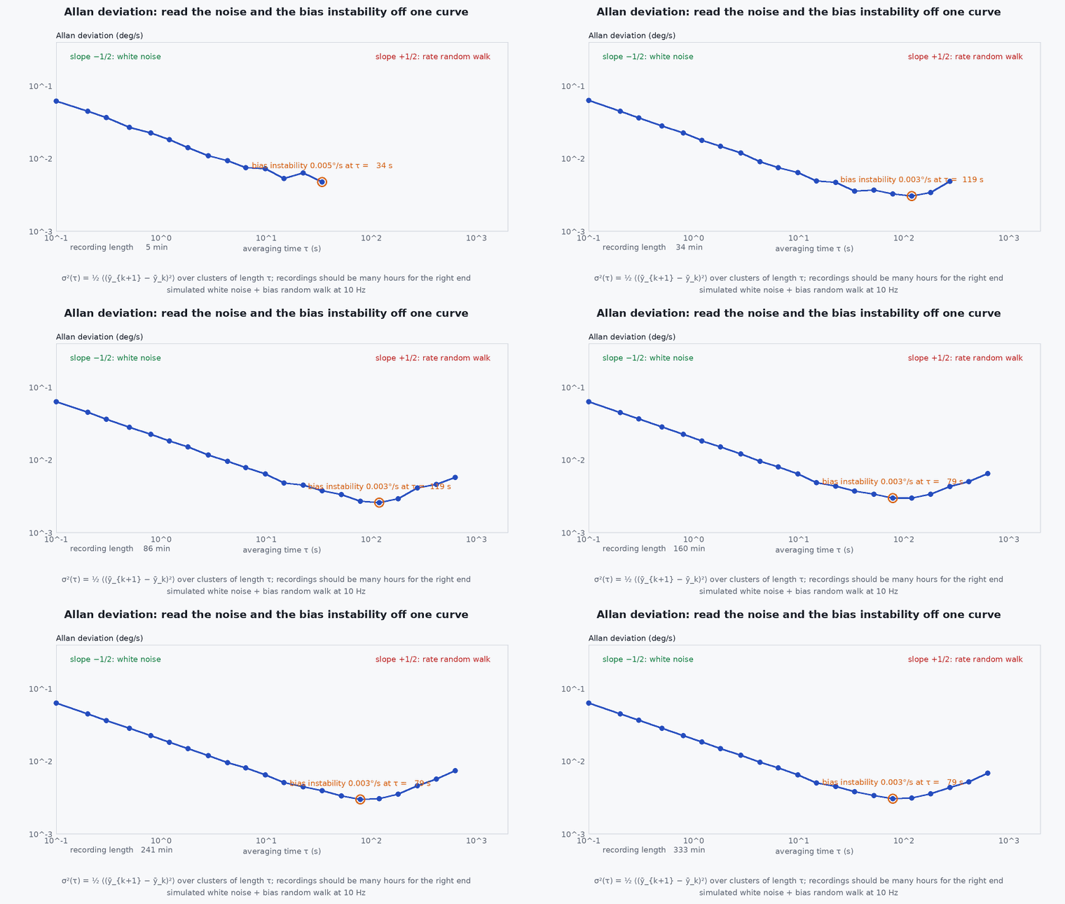
- Read noise density and random walk from an Allan deviation plot.
- Discretise continuous noise parameters for a given sample time.
- Estimate parameters from a stationary log in code.
Conceptual explanation
A raw IMU measurement is the true signal plus a slowly changing bias plus white noise. Two parameters per sensor are the minimum: the noise density (units: m/s²/√Hz for the accelerometer, rad/s/√Hz for the gyro) and the bias random-walk (rad/s²/√Hz for a gyro). A third, bias instability, is the best-case flicker floor of the bias and is read from the minimum of the Allan deviation.
Engineering intuition
Averaging white noise helps: the error shrinks as the square root of averaging time. Bias does not average away; it wanders. The Allan deviation plots the stability of the signal against averaging time: it falls while noise is being averaged, bottoms out where the wandering bias starts to dominate, and rises after. That minimum is the longest you can usefully average a stationary sensor; filters use the two ends of the plot as their noise and random walk parameters.
Mathematical formulation
Continuous-time model for a gyro (the accelerometer is identical):
- noise density (rad/s/√Hz): variance of the sampled noise is .
- bias random-walk density (rad/s²/√Hz): the bias variance grows as .
- sample period.
Discrete-time equivalents for a filter at sample time :
Allan deviation
These relations are from IEEE Std 952 and its derivatives. Vendors sometimes quote noise in or µg/√Hz: convert carefully (1°/√h = (1/60) °/s/√Hz ≈ rad/s/√Hz), and treat datasheet values as lower bounds. Measure your own unit.
Architecture and data flow
Allan-derived parameters feed the filter’s process-noise matrix : the noise density sets the covariance growth of attitude and velocity per step; the random-walk densities set how fast the bias states are allowed to wander (and so how responsive bias estimation is). In VIO configuration files these are exactly the four parameters (accelerometer and gyro noise and random walk). Inflating them modestly above the measured values is common and absorbs unmodelled effects such as vibration; inflate on evidence, not fear.
Real-world UAV applications
- Configuring VINS-Fusion, OpenVINS and similar systems (they ask for these four numbers).
- Choosing an IMU: comparing candidate sensors on the parameter that matters for your outage duration.
- Building simulations with realistic IMU errors.
- Detecting a damaged or temperature-sensitive IMU by comparing its Allan curve to its history.
Implementation example
This runs as shown: it simulates a gyro with known white noise and bias random walk, computes the overlapping Allan deviation, and recovers the noise density and the random walk from the two ends of the curve.
import numpy as np
rng = np.random.default_rng(7)
fs = 100.0; dt = 1 / fs; n = 1_000_000                       # 10 000 s of stationary data at 100 Hz
N_true = 0.002                                                # noise density (rad/s/sqrt(Hz))
K_true = 1e-4                                                 # bias random walk (rad/s^2/sqrt(Hz)): large, to show the random-walk region
white = N_true / np.sqrt(dt) * rng.standard_normal(n)
bias = np.cumsum(K_true * np.sqrt(dt) * rng.standard_normal(n))
y = white + bias                                              # stationary gyro output

def allan_dev(y, m):                                          # non-overlapping clusters of m samples
    k = len(y) // m
    means = y[: k * m].reshape(k, m).mean(axis=1)
    return np.sqrt(0.5 * np.mean(np.diff(means) ** 2))

tau_s = np.array([1, 3, 10, 30, 100, 300])                    # averaging times in seconds
ad = np.array([allan_dev(y, int(t * fs)) for t in tau_s])
N_est = ad[0] * np.sqrt(tau_s[0])                             # white-noise region (slope -1/2): N = sigma_A * sqrt(tau)
K_est = ad[-1] * np.sqrt(3.0 / tau_s[-1])                     # random-walk region (slope +1/2): K = sigma_A * sqrt(3 / tau)
print(f"N: true {N_true:.4f}, estimated {N_est:.4f} | K: true {K_true:.1e}, estimated {K_est:.1e}")
assert abs(N_est / N_true - 1) < 0.15
assert 0.5 < K_est / K_true < 2.0 # long-tau Allan estimates from one run are noisyCommon engineering mistakes
Using datasheet noise density as is
Datasheets are typically at best-case temperature and without vibration. Measure on the vehicle, motors off, then with motors on.
Mixing units
µg/√Hz vs m/s²/√Hz and vs rad/s/√Hz are the usual disasters. Write units on every parameter.
Treating bias as constant in the filter
Without a random walk the filter cannot track bias changes and drift returns after warm-up.
Calibrating on a table with motors off and flying with motors on
Vibration adds noise and bias (rectification) that the stationary test does not capture.
Inflating noise by orders of magnitude to “make it work”
This usually hides a timing or extrinsics bug.
Failure modes
| Failure mode | How it shows up | Likely cause |
|---|---|---|
| Too-small accelerometer noise in a VIO config | Filter trusts IMU too much, drifts when vision is lost | Datasheet noise used without margin for vibration |
| Too-large noise | Filter ignores the IMU, jittery estimate | Overcautious inflation |
| Bias estimate oscillates | Bias state moves rapidly with the motion | Random walk set too high or observability poor |
| Temperature-correlated drift | Bias changes with warm-up | No thermal model and heating from the companion |
Debugging approach
- Record 2–3 hours stationary at constant temperature and compute the Allan deviation of each axis.
- Repeat with motors spinning (props off) to see vibration’s effect on noise.
- Check that estimated biases in flight stay within a reasonable band; a bias state that saturates points to a wrong model elsewhere.
- Compare Allan curves between units: a mismatch indicates a damaged or different sensor revision.
Practical exercises
- Convert 100 µg/√Hz to m/s²/√Hz and 0.1°/√h to rad/s/√Hz.
- For a 200 Hz IMU with N = 0.003 m/s²/√Hz, find the standard deviation of one sample.
- Compute the growth of position uncertainty after 10 s from white accelerometer noise alone.
- Run the code with ten times larger and observe the Allan curve.
Interview questions
Write an answer in your own words, then reveal the model answer. Nothing is sent anywhere.
Question 1
What is the difference between noise density and bias random walk?
Model answer
Noise density sets sample-to-sample white noise (error shrinks by averaging); bias random walk sets how fast the slowly varying offset wanders (error grows with time). They show up on opposite ends of the Allan plot.
Question 2
Why is bias instability read at the minimum of the Allan curve?
Model answer
At short times white noise dominates and averaging helps; at long times the random walk dominates; the minimum is where the bias flicker floor is the limiting error.
Question 3
Why do VIO systems need IMU noise parameters?
Model answer
They set the covariance of IMU preintegration and of bias evolution, which weights IMU against vision in the optimisation. Wrong values mis-weight the sensors.
References and further reading
Primary papers, official documentation and standards. Each claim above that is specific to a tool or version points here.
- IEEE Std 952-1997: Guide for the specification of inertial sensors (Allan variance); check for the current revision
- D. W. Allan, “Statistics of atomic frequency standards”, Proceedings of the IEEE, 1966
- allan_variance_ros: IMU noise parameter estimation tool for ROS
- OpenVINS documentation: IMU noise parameter configuration