UAV Systems Engineering · Module 3
M3-T5: Extended Kalman Filter
When the world is nonlinear, linearise at the current estimate: the EKF is the Kalman filter with Jacobians in place of matrices.
UAV models are nonlinear: attitude rotations, bearing and range measurements, camera projections. The EKF handles them by linearising at each step. It works well when uncertainty is small, and it fails in ways that are worth knowing before you trust it.
Learning objectives
After this lesson, you should be able to:
- State the EKF equations and the role of the Jacobians.
- Derive the Jacobian of a range-bearing measurement model.
- Verify Jacobians numerically with finite differences.
- Explain EKF inconsistency and the situations that cause it.
Conceptual explanation
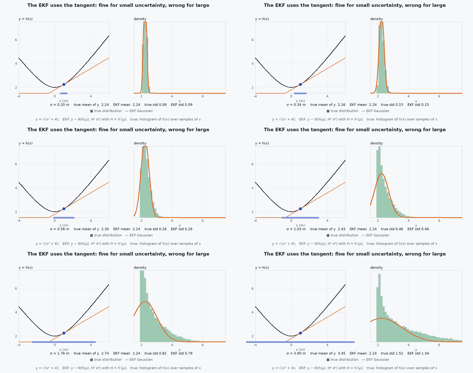
The Kalman filter needs linear models. The EKF replaces the nonlinear motion and measurement with their first-order Taylor expansions around the current estimate. The matrices and (the Jacobians) take the place of the constant matrices, and the covariance is propagated through them exactly as before. The state is propagated through the full nonlinear function; only the covariance uses the linearisation.
Engineering intuition
If the estimate is uncertain by ±1 m and the function curves gently over that range, the tangent is nearly the function and the EKF is nearly exact. If the uncertainty is large relative to the curvature (a poor initial guess, a bearing measurement to a nearby object, a heading error of tens of degrees) the tangent is a poor stand-in. The covariance then no longer describes the true error, the filter becomes overconfident, and it can diverge. The cure is not bigger numbers but better linearisation points, better initial estimates, or a different filter (error-state, iterated, unscented).
Mathematical formulation
Model: , .
Range and bearing
For a station at the origin and a vehicle at (, ), the measurement is . With :
The bearing innovation must be wrapped to : .
Checking Jacobians
Most EKF bugs live in the Jacobians. Check them numerically in a test, always.
Architecture and data flow
Inside PX4, EKF2 is an error-state filter: it propagates the nominal state with the IMU and estimates small errors (lesson M3-T6). The principle, linearise at the estimate and fuse sensors sequentially with their measurement Jacobians, is the EKF’s. When you feed external odometry, you are supplying a measurement with a covariance that the filter uses exactly as in the update above.
Real-world UAV applications
- GNSS/INS fusion in autopilots.
- Bearing-only and range-bearing target tracking.
- Camera-based measurement updates (reprojection residuals) in MSCKF-style VIO.
- Landing on a beacon using range and bearing.
Implementation example
This runs as shown: it verifies the analytic Jacobians with finite differences and runs an EKF on range-bearing tracking, reporting the position error and NIS consistency.
import numpy as np
rng = np.random.default_rng(5)

def h(x):  return np.array([np.hypot(x[0], x[1]), np.arctan2(x[1], x[0])])
def H_of(x):
    r = np.hypot(x[0], x[1])
    return np.array([[x[0]/r, x[1]/r, 0, 0], [-x[1]/r**2, x[0]/r**2, 0, 0]])

# 1) Jacobian check by central differences
x0 = np.array([30.0, 20.0, 3.0, -1.0]); eps = 1e-6
Hn = np.column_stack([(h(x0 + eps*e) - h(x0 - eps*e)) / (2*eps) for e in np.eye(4)])
assert np.allclose(Hn, H_of(x0), atol=1e-7)

# 2) EKF on a constant-velocity target
dt, n = 0.2, 300
F = np.eye(4); F[0, 2] = F[1, 3] = dt
q = 0.3; Qb = q * np.array([[dt**3/3, dt**2/2], [dt**2/2, dt]])
Q = np.zeros((4, 4)); Q[np.ix_([0, 2], [0, 2])] = Qb; Q[np.ix_([1, 3], [1, 3])] = Qb
R = np.diag([1.5**2, np.radians(1.0)**2])
Lq = np.linalg.cholesky(Q + 1e-12*np.eye(4))
xt = np.array([60.0, 25.0, -2.0, 1.0]); xh = xt + np.array([5.0, -5.0, 1.0, 1.0]); P = np.diag([25.0, 25.0, 4.0, 4.0])
nis, errs = [], []
for k in range(n):
    xt = F @ xt + Lq @ rng.standard_normal(4)
    z = h(xt) + np.sqrt(np.diag(R)) * rng.standard_normal(2)
    xh = F @ xh; P = F @ P @ F.T + Q
    H = H_of(xh); y = z - h(xh); y[1] = (y[1] + np.pi) % (2*np.pi) - np.pi        # wrap the bearing innovation
    S = H @ P @ H.T + R; K = P @ H.T @ np.linalg.inv(S)
    xh = xh + K @ y; I_KH = np.eye(4) - K @ H; P = I_KH @ P @ I_KH.T + K @ R @ K.T
    if k > 30: nis.append(y @ np.linalg.inv(S) @ y); errs.append(np.hypot(*(xh[:2] - xt[:2])))
print(f"mean position error {np.mean(errs):.2f} m, mean NIS {np.mean(nis):.2f} (expected 2)")
assert np.mean(errs) < 3.0 and 1.2 < np.mean(nis) < 3.2Common engineering mistakes
Wrong or unchecked Jacobians
Verify with finite differences in a unit test.
Forgetting to wrap angle innovations
bearing error instead of − wrecks the update.
Linearising at a poor initial guess
A far-off start produces an unrepresentative Jacobian and divergence; initialise with a robust method, then switch to the EKF.
Compensating inconsistency by inflating noise blindly
It hides the problem. Diagnose with NIS and NEES.
Using the EKF for large attitude errors with Euler angles
Use an error-state formulation with quaternions.
Failure modes
| Failure mode | How it shows up | Likely cause |
|---|---|---|
| Linearisation error | Filter is confidently wrong when uncertainty is large | Bad initialisation, nearby bearing measurements, large heading error |
| Angle wrap bug | Sudden state jump when the bearing crosses ± | Innovation not wrapped |
| Inconsistency | NEES far above its expected value | Linearisation or unmodelled error; overconfident covariance |
| Singularity | NaN near | Division by range in the Jacobian |
Debugging approach
- Compare analytic and numerical Jacobians at several operating points including extreme ones.
- Run the filter in simulation with exactly known noise; fix inconsistency there before real data.
- Plot angle innovations and verify they stay within and look white.
- Start the filter from several initial guesses and check it converges from all.
Practical exercises
- Derive the Jacobian for a bearing-only measurement and discuss observability from a single station.
- Use the EKF Simulator to find the smallest that keeps NIS in its 95% bounds on the manoeuvring target.
- Increase the initial position error to 40 m with an initial of 1 m and report what happens.
- Replace the EKF update by an iterated update (relinearise 3 times) and compare consistency.
Interview questions
Write an answer in your own words, then reveal the model answer. Nothing is sent anywhere.
Question 1
How does the EKF differ from the Kalman filter?
Model answer
It linearises the nonlinear process and measurement models at the current estimate using Jacobians. The state goes through the nonlinear functions; the covariance goes through their linearisations.
Question 2
When does the EKF fail?
Model answer
When uncertainty is large compared with the nonlinearity (poor initialisation, strong curvature), producing overconfident covariance and divergence; also from wrong Jacobians or unwrapped angles.
Question 3
How do you verify an EKF implementation?
Model answer
Check Jacobians against finite differences, test on simulated data with known noise, and check NIS/NEES against chi-square expectations.
References and further reading
Primary papers, official documentation and standards. Each claim above that is specific to a tool or version points here.
- . . Barfoot, State Estimation for Robotics, Cambridge University Press, 2017, chapter 4.
- . Bar-Shalom, . . Li, . Kirubarajan, Estimation with Applications to Tracking and Navigation, Wiley, 2001, chapter 5.
- PX4: Using the EKF2 estimator