UAV Systems Engineering · Module 4
M4-T10: FAST-LIVO2
FAST-LIVO2 applies the LiDAR update and then the camera update to the same iterated filter, using the LiDAR map to supply the depth that the image patches need.
FAST-LIVO2 (Zheng et al., IEEE T-RO 2025) extends FAST-LIO2 with a camera in a direct, photometric way. It is a research system whose design is instructive for any UAV that wants LiDAR geometry and visual texture in one estimator at a modest compute cost.
Learning objectives
After this lesson, you should be able to:
- Describe the FAST-LIVO2 structure: ESIKF with sequential LiDAR then visual update and a unified voxel map.
- Explain direct photometric alignment of image patches and why LiDAR depth is needed.
- Show that sequential and joint updates of independent measurements agree in the linear case.
- State the assumptions: calibration, synchronisation, exposure and a static scene.
Conceptual explanation
The description follows the FAST-LIVO2 paper (arXiv:2408.14035) and repository; details such as parameter names and supported sensors belong to the repository for your version.
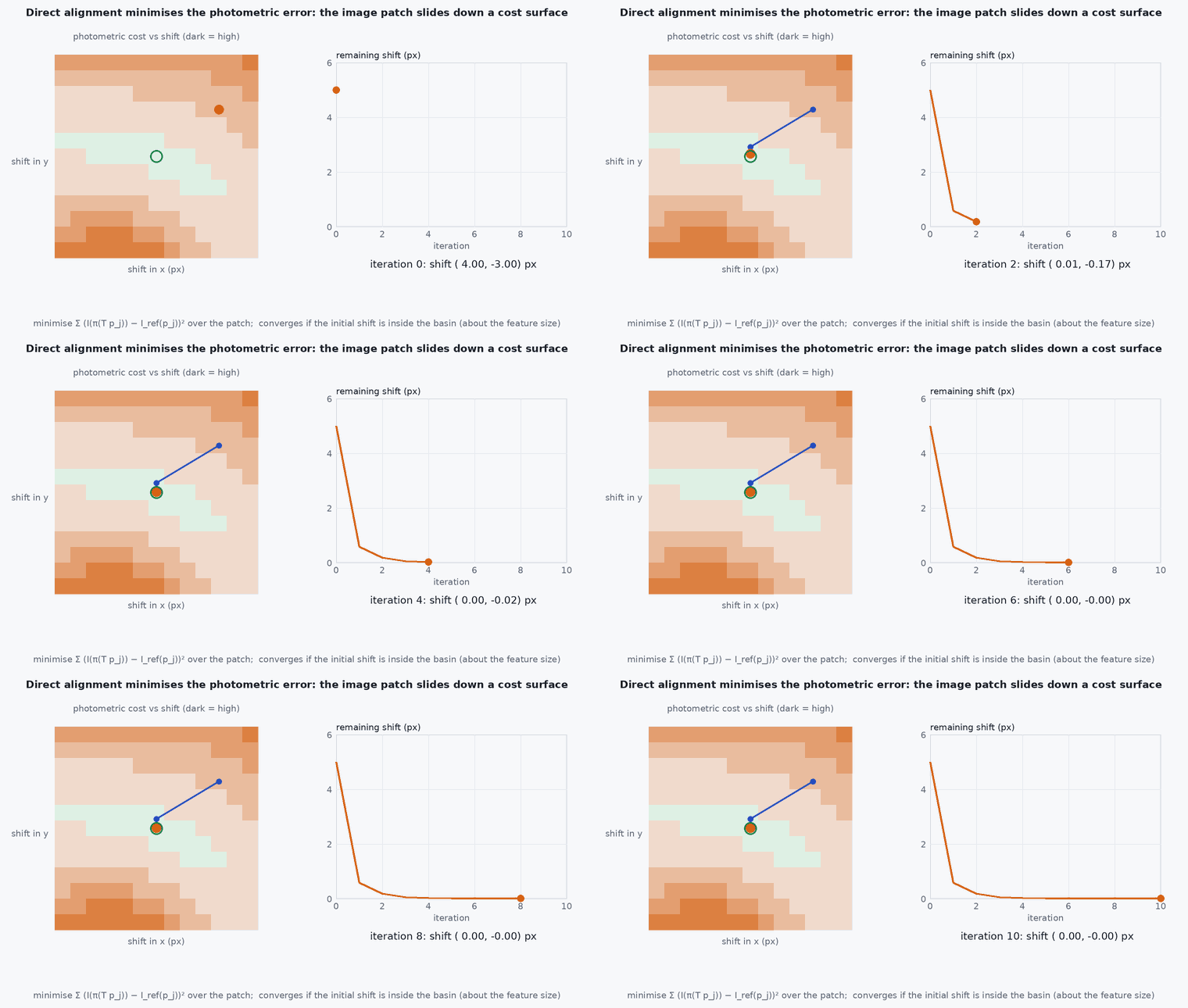
FAST-LIVO2 is a direct method: it does not extract geometric or visual features; the LiDAR registers raw points to planes in a voxel map, and the camera aligns small image patches attached to map points by minimising photometric error. The state estimator is an error-state iterated Kalman filter (ESIKF) that processes the LiDAR measurement first and the image measurement second (a sequential update) within one filter step, avoiding a high-dimensional joint update. LiDAR points give the depth of map points, so no depth has to be estimated visually; on-demand ray casting and reference patch updating handle occlusion and viewpoint change; camera exposure time is estimated online to cope with lighting changes.
Engineering intuition
Feature-based vision spends effort finding and matching features and estimating their depth. FAST-LIVO2 spends none: the map points already have accurate depth from the LiDAR and each carries a small image patch seen at a previous view; the update simply asks how the pose must change for the new image to look like the stored patch. That is cheap and does not need texture to look like corners: any gradient helps. The price is sensitivity to brightness changes (hence exposure estimation) and to calibration: a misaligned camera–LiDAR extrinsic puts the patch in the wrong place.
Mathematical formulation
Photometric residual for a map point with 3-D position (from the LiDAR map), reference patch intensities and the current image I with pose and exposure ratio :
Sequential update: for independent measurements , with models , and noise , , updating with and then gives the same posterior as a joint update with the stacked measurement (when the measurements are conditionally independent and the model is linear):
In the nonlinear iterated case the equivalence is approximate but the sequential form is much cheaper because each update has a smaller measurement dimension. Computational note from the paper: the filter state dimension, not the number of residuals, dominates the cost.
- map point position, with depth from the LiDAR map.
- exposure scale factor estimated online.
- camera pose from the filter state.
Architecture and data flow
Inputs: LiDAR with per-point times, IMU, camera images, calibrated extrinsics (camera–LiDAR–IMU) and camera intrinsics; the repository documents the configuration for supported sensor setups. Outputs: odometry, a coloured point cloud map and per-sensor status. For a UAV, budget compute carefully (the paper reports operation on embedded platforms with a variant for resource-constrained devices: check the publication list in the repository) and verify timing on your computer (lesson M7-T3).
Real-world UAV applications
- LiDAR-camera-IMU odometry in mixed environments (Capstone 4 option).
- Coloured mapping and visual inspection data registered to LiDAR geometry.
- Studying sequential updates and direct methods.
- A reference for deciding between feature-based and direct VIO.
Implementation example
This runs as shown: two independent linear measurements are applied to a Kalman filter jointly and sequentially, giving the same posterior to machine precision, and the sequential form needs only small matrix inversions.
import numpy as np
rng = np.random.default_rng(1)
n = 6
x0 = np.zeros(n); P0 = np.diag(rng.uniform(0.5, 2.0, n))
H1 = rng.standard_normal((4, n)); R1 = np.diag(rng.uniform(0.05, 0.2, 4))       # "LiDAR" measurement (4 residuals)
H2 = rng.standard_normal((3, n)); R2 = np.diag(rng.uniform(0.05, 0.2, 3))       # "camera" measurement (3 residuals)
z1 = rng.standard_normal(4); z2 = rng.standard_normal(3)

def update(x, P, z, H, R):
    S = H @ P @ H.T + R; K = P @ H.T @ np.linalg.inv(S)
    return x + K @ (z - H @ x), (np.eye(len(x)) - K @ H) @ P

# joint update with the stacked measurement
Hj = np.vstack([H1, H2]); Rj = np.block([[R1, np.zeros((4, 3))], [np.zeros((3, 4)), R2]])
xj, Pj = update(x0, P0, np.concatenate([z1, z2]), Hj, Rj)
# sequential: LiDAR first, then the camera
xs, Ps = update(x0, P0, z1, H1, R1); xs, Ps = update(xs, Ps, z2, H2, R2)
print("max difference in the mean:", np.abs(xj - xs).max(), "and in the covariance:", np.abs(Pj - Ps).max())
assert np.allclose(xj, xs, atol=1e-10) and np.allclose(Pj, Ps, atol=1e-10)
assert np.linalg.inv(H1 @ P0 @ H1.T + R1).shape == (4, 4) # sequential inversions are 4x4 then 3x3, not 7x7Common engineering mistakes
Poor camera–LiDAR extrinsics
Patches are placed wrongly and the photometric update fights the geometry.
Ignoring exposure changes and rolling shutter
Photometric residuals are biased.
Using it on a dynamic scene without care
Moving objects violate the static-map assumption.
Expecting robustness without calibration of time offsets
Direct methods are sensitive to timing.
Skipping the compute measurement
Check the real-time margin on your computer.
Failure modes
| Failure mode | How it shows up | Likely cause |
|---|---|---|
| Photometric divergence | Drift in sudden lighting changes | Exposure estimation insufficient |
| LiDAR-degenerate scene with a textureless camera view | Drift along an axis | Neither sensor constrains it |
| Calibration drift | Systematic errors after a hard landing | Mount shift |
| Overload | Frame drops | Compute budget exceeded |
Debugging approach
- Overlay projected map points on the image to check extrinsics.
- Monitor photometric error per frame and exposure estimate.
- Run LIO-only and LIVO on the same bag for an ablation.
- Profile per-stage time.
Practical exercises
- Show that sequential and joint updates differ for a nonlinear measurement and quantify it.
- Read the FAST-LIVO2 paper’s ablation on the exposure estimation and summarise it.
- Estimate the sequential versus joint update cost for 200 LiDAR residuals and 100 photometric ones.
- Decide which of FAST-LIO2 and FAST-LIVO2 to use for a vehicle that flies in a dark warehouse.
Interview questions
Write an answer in your own words, then reveal the model answer. Nothing is sent anywhere.
Question 1
What is direct in FAST-LIVO2?
Model answer
It uses raw LiDAR points and image intensities directly (point-to-plane and photometric residuals) without extracting geometric or visual features.
Question 2
Why sequential updates?
Model answer
Applying the LiDAR and then the visual update to the same iterated filter is cheaper than one joint update and equivalent for independent linear measurements.
Question 3
Why does the camera need the LiDAR map?
Model answer
The LiDAR supplies accurate depth of the map points so photometric patches need no visual depth estimation.
References and further reading
Primary papers, official documentation and standards. Each claim above that is specific to a tool or version points here.