UAV Systems Engineering · Module 4
M4-T9: Visual-LiDAR-Inertial Odometry
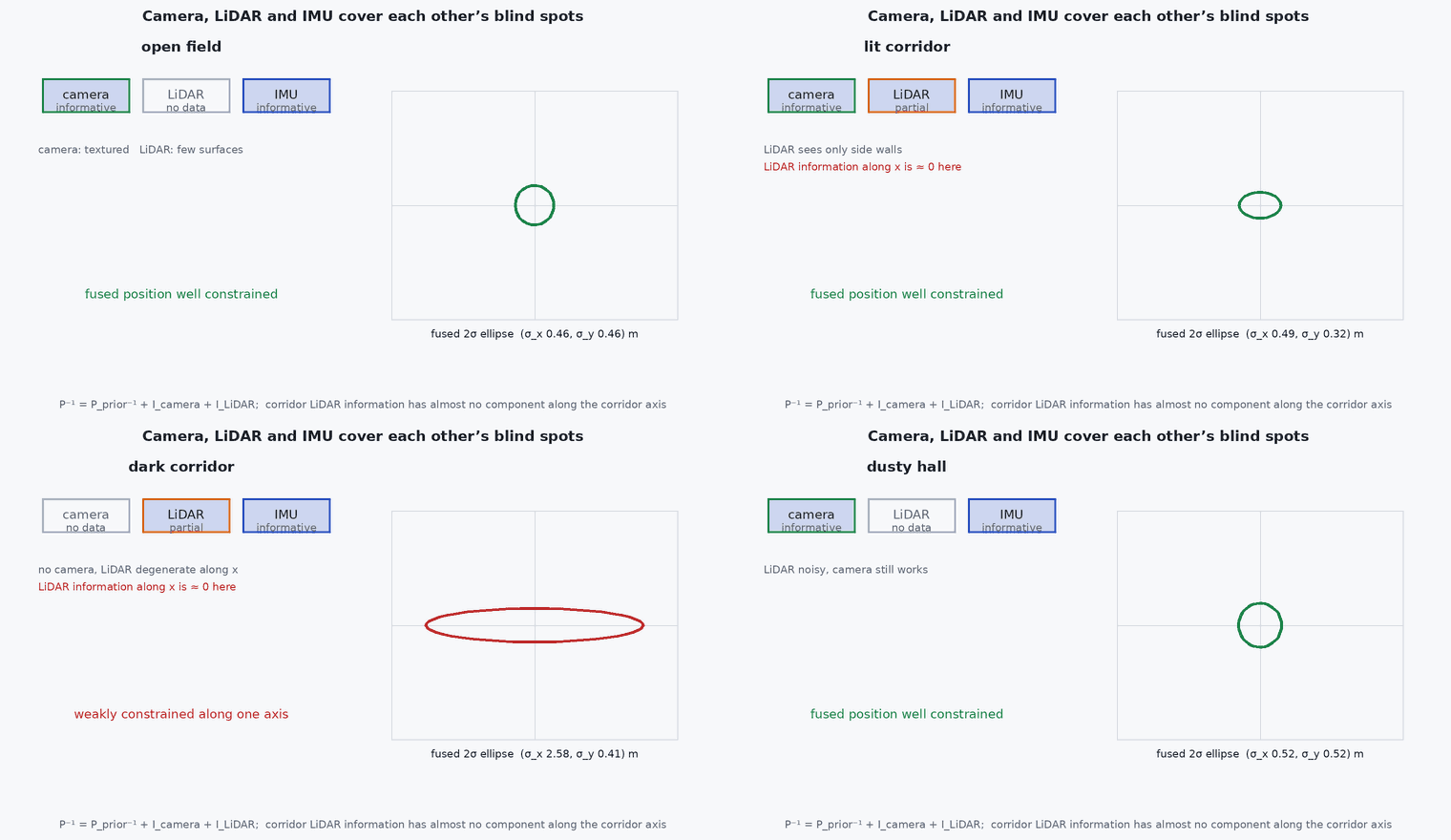
Camera gives texture and constraints in the directions where LiDAR is blind; LiDAR gives metric depth where the camera is blind: each repairs the other.
A vehicle that must survive both a dark featureless corridor and a bright geometrically bare field needs more than one exteroceptive sensor. This lesson sets out why camera, LiDAR and IMU are combined, how the combinations are structured, and what must be calibrated.
Learning objectives
After this lesson, you should be able to:
- Explain the complementary strengths and failure modes of camera and LiDAR.
- Describe loosely and tightly coupled LiDAR-visual-inertial architectures.
- Show with an information-matrix example how vision constrains a LiDAR-degenerate direction.
- List the calibration and synchronisation requirements.
Conceptual explanation
LiDAR provides accurate metric geometry independent of light but can be degenerate in structureless geometry (lesson M2-T13); a camera provides dense texture and constraints along directions that LiDAR cannot see, but needs light and texture and has no direct scale. A visual-LiDAR-inertial system uses the IMU as the common backbone: prediction, deskewing and a shared state; the exteroceptive sensors provide corrections. Examples: LVI-SAM (factor graph, two subsystems that assist each other), R3LIVE and FAST-LIVO2 (filter-based, direct).
| Condition | LiDAR | Camera | Combined |
|---|---|---|---|
| Dark corridor | good (walls) but degenerate along the axis | blind | LiDAR constrains across, IMU bridges along |
| Textured corridor with light | degenerate along the axis | good along the axis (texture) | camera constrains the LiDAR-degenerate direction |
| Open field, bright | degenerate (flat ground) | good if texture exists | camera constrains horizontal motion |
| Fog, dust | noisy returns | blind | LiDAR with filtering, radar (lesson M2-T15) |
Engineering intuition
Information is a matrix: each sensor adds a positive semi-definite contribution; a direction is well constrained if the sum has a large eigenvalue there. LiDAR may contribute nothing along the corridor; a camera looking at textured walls contributes along it. The fusion is therefore not an average but an addition of information in complementary directions. The practical rules: make sure the camera and LiDAR agree in time and extrinsics, and monitor each sensor’s own health so the fused weights follow reality (lesson M2-T16).
Mathematical formulation
Information (Fisher) form: with measurement Jacobians (LiDAR) and (camera) and noise covariances and , the information about the state is the sum:
FAST-LIVO2 (Zheng et al.) estimates with an error-state iterated Kalman filter in which the LiDAR point-to-plane update and the image photometric update are applied sequentially within the same iterated framework, with a unified voxel map whose planes also provide the depth for the photometric patches. Photometric methods additionally need exposure (brightness) handling. LVI-SAM runs a visual-inertial and a LiDAR-inertial system, each using the other’s output for initialisation and scale, with a joint factor-graph smoother.
- ,
- LiDAR and camera measurement Jacobians with respect to the state.
- ,
- noise covariances.
Architecture and data flow
Requirements: synchronised camera, LiDAR and IMU clocks (lesson M7-T8); calibrated camera intrinsics and camera–LiDAR–IMU extrinsics (lesson M7-T16); per-point LiDAR timestamps; exposure handling for photometric methods. Output: odometry with covariance and health for each sensor. Compute: a LiDAR-visual system is the heaviest of the estimators in this track; budget it (lesson M7-T12).
Real-world UAV applications
- GNSS-denied flight across mixed indoor and outdoor environments.
- The perception core of Capstone 4.
- Coloured maps and visual–geometric reconstruction.
- Redundant odometry with diverse failure modes (lesson M2-T16).
Implementation example
This runs as shown: the translational information matrix of a corridor LiDAR (degenerate along the axis) is added to the information from a camera that observes along-axis motion with a given accuracy. The along-axis standard deviation falls from effectively unbounded to the camera’s level, while the other directions stay LiDAR-accurate.
import numpy as np
rng = np.random.default_rng(0)
# LiDAR in a corridor along x: surface normals are only along y and z, so the x direction carries no information
normals = np.vstack([np.tile([0, 1.0, 0], (300, 1)), np.tile([0, 0, 1.0], (300, 1))]) + 0.01 * rng.standard_normal((600, 3)) * np.array([0, 1.0, 1.0])
normals /= np.linalg.norm(normals, axis=1, keepdims=True)
sigma_L = 0.03
I_lidar = normals.T @ normals / sigma_L ** 2

# camera: tracks texture on the walls; observes motion along the corridor with about 5 cm accuracy per frame and little across
I_cam = np.diag([1 / 0.05 ** 2, 1 / 0.5 ** 2, 1 / 0.5 ** 2])


cov_lidar = np.linalg.inv(I_lidar + 1e-9 * np.eye(3)); cov_both = np.linalg.inv(I_lidar + I_cam)
s_l, s_b = np.sqrt(np.diag(cov_lidar)), np.sqrt(np.diag(cov_both))
print("std (x along, y, z) LiDAR only :", np.round(s_l, 3)); print("std (x along, y, z) LiDAR + cam:", np.round(s_b, 4))
assert s_l[0] > 1000 * s_l[1]                                      # LiDAR alone: the along-corridor direction is unconstrained (huge standard deviation)
assert s_b[0] < 0.06 and s_b[1] < s_l[1] and abs(s_b[0] - 0.05) < 0.01   # the camera pins the along direction to about its own accuracy
assert s_b[1] < 0.03 and s_b[2] < 0.03 # the other directions remain LiDAR-accurateCommon engineering mistakes
Fusing both with equal weight regardless of health
A blind camera in the dark or a degenerate LiDAR must be down-weighted automatically.
Camera–LiDAR extrinsics from a rough guess
Photometric methods are especially sensitive to them.
Ignoring exposure changes
Photometric residuals are biased by brightness changes.
Treating the system as redundant when failures are correlated
Darkness and dust can defeat both together; add radar.
Underestimating compute
It is the most expensive estimator: measure it on the target.
Failure modes
| Failure mode | How it shows up | Likely cause |
|---|---|---|
| Sensor conflict | Odometry jumps when one sensor degrades | No health-based weighting |
| Photometric failure | Drift when lighting changes | Exposure not modelled |
| Calibration error | Systematic drift or smeared map | Extrinsics or time offset wrong |
| Common-mode failure | Both sensors fail together | Dust, fog or darkness plus geometric degeneracy |
Debugging approach
- Plot the information eigenvalues for each sensor in time.
- Verify camera–LiDAR extrinsics by projecting the point cloud on the image.
- Run ablations: LIO only, VIO only, both.
- Check exposure compensation on a lighting-change sequence.
Practical exercises
- Compute the information matrix for a camera that looks at a wall ahead and one that looks down.
- Evaluate an ablation: LIO only versus LIVO on a public dataset with a corridor.
- List the extra calibration needed beyond LIO.
- Decide whether to add radar to your design for a dust-prone environment.
Interview questions
Write an answer in your own words, then reveal the model answer. Nothing is sent anywhere.
Question 1
Why combine camera and LiDAR?
Model answer
Their failure modes are complementary: LiDAR is geometric and light-independent but can be degenerate, cameras are texture-based and fill degenerate directions but need light.
Question 2
How does information addition explain the benefit?
Model answer
Each sensor adds a positive semi-definite information matrix; a direction unconstrained by LiDAR can be constrained by the camera, so the sum has no small eigenvalue.
Question 3
What is the main extra calibration burden?
Model answer
Camera–LiDAR–IMU extrinsics and time offsets, and for photometric methods, camera exposure.
References and further reading
Primary papers, official documentation and standards. Each claim above that is specific to a tool or version points here.