UAV Systems Engineering · Module 3
M3-T13: Innovation monitoring
If the filter is right, its innovations are white noise: any pattern in them is information about what is wrong.
The innovation is the filter’s surprise at each measurement. It is available in flight without ground truth, which makes it the main online health indicator. This lesson shows what an honest innovation sequence looks like and how to read the patterns that dishonesty leaves.
Learning objectives
After this lesson, you should be able to:
- Define the innovation and state the properties of a consistent filter’s innovation sequence.
- Test for zero mean, correct variance and whiteness.
- Diagnose bias, wrong noise levels and unmodelled dynamics from innovation patterns.
- Implement an online innovation monitor.
Conceptual explanation
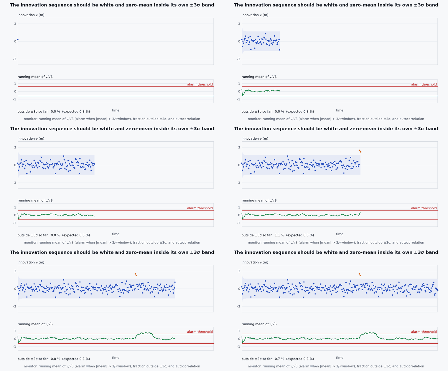
The innovation is the part of the measurement the filter did not predict. For an optimal filter with correct models, the innovation sequence is zero-mean, has covariance and is white (uncorrelated in time): nothing predictable remains.
Engineering intuition
Think of the innovations as the residue of a fit. If a model captured everything predictable, the residue is noise. A drifting residue means the model misses a slowly varying effect (a bias); a residue that oscillates with the manoeuvres means the model dynamics are wrong (a missing term, a delay); a residue that is white but too large means the noise values are too small. Each pattern points at a different fix, which is why plotting the innovation is the first debugging step for a misbehaving estimator.
Mathematical formulation
Tests for a scalar innovation sequence with predicted variances (normalised ):
Limit: a constant bias on the only sensor that observes a state is absorbed into the state estimate and leaves the innovations healthy: it is unobservable. Detecting it needs a second, independent source (lesson M2-T6, M3-T16). Interpretation: a significantly non-zero mean means a recent change or a bias against the model; a normalised variance well above 1 (below 1) means R or Q too small (large); significant autocorrelation at lag τ points to dynamics on the time scale τ, or a time delay of that order. These tests use a window of recent data and are reported with the sample size, so that their statistical power is known.
- νk
- normalised innovation.
- ρ(τ)
- sample autocorrelation at lag τ.
- N
- window length (number of innovations).
Architecture and data flow
Each update emits (time, source, innovation, ); the monitor keeps a sliding window per source, computes mean, variance and autocorrelation, and publishes a status: healthy, biased, noisy, or lagging. PX4’s EKF2 publishes innovations and their test ratios (estimator status and innovation topics) that you can plot in the (lesson M6-T13).
Real-world UAV applications
- Tuning and from logs without ground truth.
- Detecting a drifting barometer or magnetometer in flight.
- Detecting a camera-IMU time offset through autocorrelated innovations.
- Feeding the health record of the navigation manager.
Implementation example
This runs as shown: a monitor classifies the innovation patterns of four filters on the same data: correct, biased measurement, noise underestimated, and a one-step measurement delay.
import numpy as np
rng = np.random.default_rng(1)
dt, n = 0.1, 3000
F = np.array([[1, dt], [0, 1]]); H = np.array([[1.0, 0.0]]); q = 0.5; r_std = 1.0
Q = lambda qq: qq * np.array([[dt**3 / 3, dt**2 / 2], [dt**2 / 2, dt]])
L = np.linalg.cholesky(Q(q)); x = np.array([0.0, 2.0]); truth = []
for _ in range(n): x = F @ x + L @ rng.standard_normal(2); truth.append(x[0])
truth = np.array(truth)

def run(zseries, q_f=q, r_f=r_std):
    xh = np.array([0.0, 2.0]); P = np.eye(2); nu = []
    for z in zseries:
        xh = F @ xh; P = F @ P @ F.T + Q(q_f); S = (H @ P @ H.T)[0, 0] + r_f ** 2; y = z - xh[0]; nu.append(y / np.sqrt(S))
        K = (P @ H.T / S).ravel(); xh = xh + K * y; P = (np.eye(2) - np.outer(K, H)) @ P
    return np.array(nu)

def monitor(nu):
    N = len(nu); m = nu.mean(); v = np.mean(nu ** 2)
    rho = [np.sum(nu[:-t] * nu[t:]) / np.sum(nu ** 2) for t in range(1, 6)]
    status = []
    if abs(m) > 3 / np.sqrt(N): status.append("bias")
    if v > 1.3: status.append("noise too optimistic")
    if v < 0.7: status.append("noise too pessimistic")
    if max(abs(r) for r in rho) > 3 / np.sqrt(N): status.append("correlated: dynamics or delay")
    return status or ["healthy"]

z_ok = truth + r_std * rng.standard_normal(n)
z_step = z_ok.copy(); z_step[1500:] += 3.0                              # a 3 m step in the measurement halfway through
nu_step = run(z_step)
cases = {
    "correct": monitor(run(z_ok)),
    "constant 0.5 m bias on the only sensor": monitor(run(z_ok + 0.5)),
    "3 m step, 60 samples after it": monitor(nu_step[1500:1560]),
    "R set too small (0.4x)": monitor(run(z_ok, r_f=0.4 * r_std)),
    "Q set too small (0.05x)": monitor(run(z_ok, q_f=0.05 * q)),
}
for k, v in cases.items(): print(f"{k:42s} -> {v}")
assert cases["correct"] == ["healthy"]
assert cases["constant 0.5 m bias on the only sensor"] == ["healthy"]        # absorbed by the position state: the innovations cannot see it
assert "noise too optimistic" in cases["3 m step, 60 samples after it"]       # a sudden change is visible, but only briefly
assert "noise too optimistic" in cases["R set too small (0.4x)"] and "correlated: dynamics or delay" in cases["Q set too small (0.05x)"]Common engineering mistakes
Looking at innovations only as outliers
The mean and correlation carry the diagnosis.
Short windows with strict thresholds
False alarms: choose from the effect size to detect.
Using normalised innovations with a wrong S
The test then checks the covariance too: that is intended, but be aware.
Tuning to make innovations white at the cost of unrealistic Q
Whiteness is necessary, not sufficient.
Ignoring that gating changes statistics
Rejected measurements bias the accepted innovation distribution.
Failure modes
| Failure mode | How it shows up | Likely cause |
|---|---|---|
| Slow bias | Mean innovation drifts away from zero | Sensor drift or an unmodelled state |
| Oscillating innovations | Autocorrelation at the manoeuvre period | Model dynamics wrong |
| Persistently large innovations | Normalised variance well above one | Noise too optimistic or a hidden fault |
| Innovation spikes at mode changes | Large values when sensors switch | Reference frame or initialisation transients |
Debugging approach
- Plot normalised innovations with ±2 bounds and their autocorrelation.
- Compare the monitor’s verdict for each sensor in the same flight.
- Vary the time offset and see the autocorrelation shift.
- Use the EKF Simulator to produce each pattern on purpose.
Practical exercises
- Choose to detect a bias at 95% power.
- Show that a one-step delay produces correlation at lag one in the example.
- Extend the monitor to a 2-D innovation using Mahalanobis distance.
- Locate the innovation topics in a PX4 log and plot one.
Interview questions
Write an answer in your own words, then reveal the model answer. Nothing is sent anywhere.
Question 1
What properties does the innovation of a consistent filter have?
Model answer
Zero mean, covariance ⁻ as predicted by the filter, and whiteness in time (no autocorrelation), because nothing predictable should remain in the residual.
Question 2
What does a correlated innovation sequence suggest?
Model answer
Unmodelled dynamics on that time scale, or a time delay between the measurement and its prediction.
Question 3
Why is innovation monitoring valuable in flight?
Model answer
It needs no ground truth and reveals bias, noise and model errors online.
References and further reading
Primary papers, official documentation and standards. Each claim above that is specific to a tool or version points here.
- . Bar-Shalom, . . Li, . Kirubarajan, Estimation with Applications to Tracking and Navigation, Wiley, 2001, chapter 5.
- . Kailath, “An innovations approach to least-squares estimation. Part I”, IEEE Transactions on Automatic Control, 1968.
- PX4: innovation test ratios and EKF2 tuning