UAV Systems Engineering · Module 3
M3-T14: Normalized Innovation Squared
If the filter is honest, its innovations are small in a known statistical sense; NIS is the number that checks it, one measurement at a time.
A filter reports its own uncertainty. NIS asks whether the measurements agree with it. It is the cheapest, most useful online health check an estimator has, and it works without ground truth.
Learning objectives
After this lesson, you should be able to:
- Define NIS and state its distribution for a consistent filter.
- Choose gating and consistency thresholds from the chi-square distribution.
- Use NIS for measurement gating and a windowed NIS for filter-health monitoring.
- Detect an injected sensor fault with NIS and measure detection delay.
Conceptual explanation
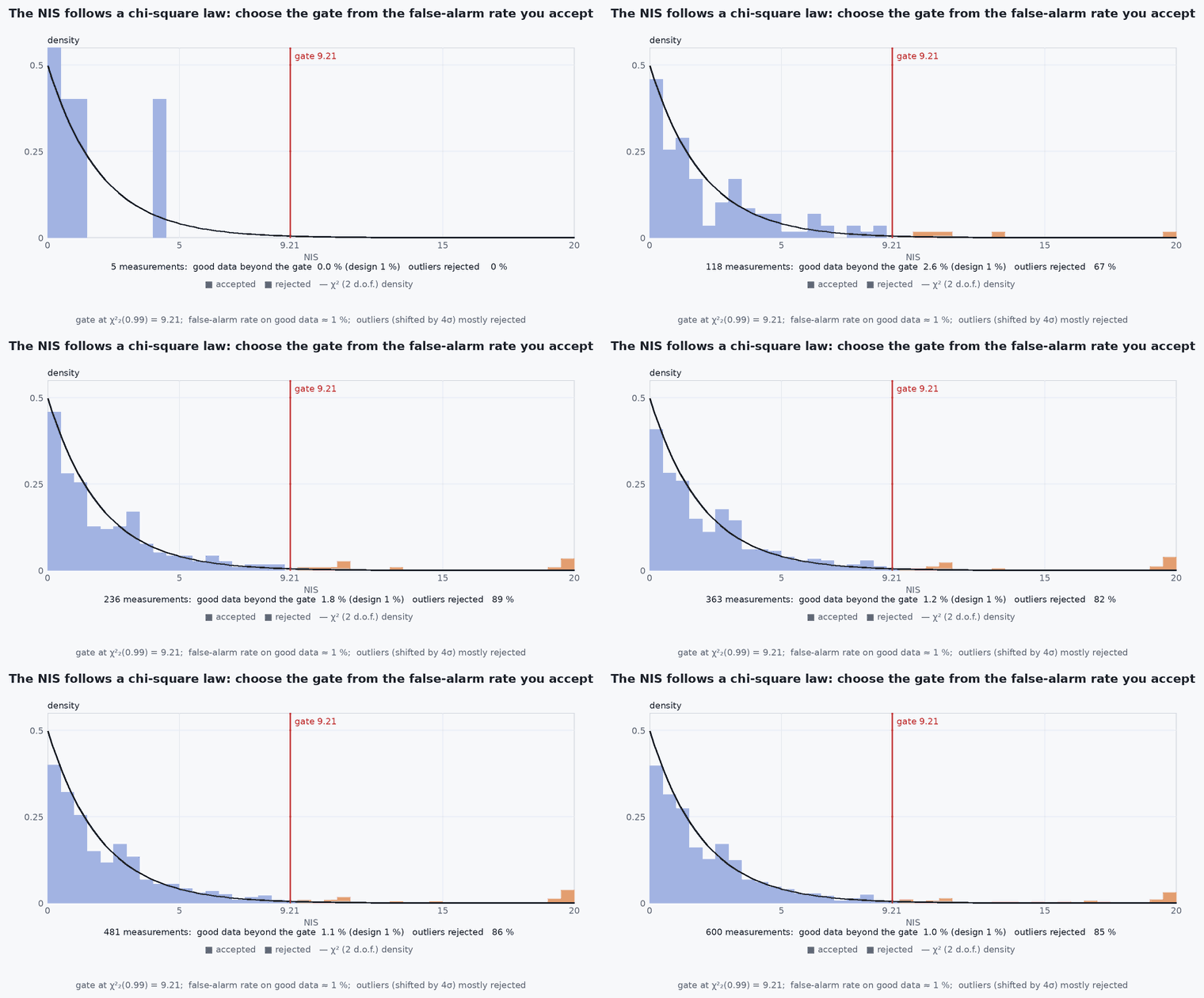
At each update the filter predicts the measurement and compares it to the real one. The difference is the innovation . If the model and noise parameters are right, is zero-mean Gaussian with covariance . The normalised innovation squared, NIS = , then follows a chi-square distribution with as many degrees of freedom as the measurement has dimensions.
Engineering intuition
The innovation is the filter’s “surprise”. NIS expresses it in units of how surprised the filter said it would be. If you tell the filter its measurements have 1 m noise and they actually have 3 m, NIS runs about nine times too high; if the prediction is biased, NIS rises as the bias grows. If you set far too large, NIS sits far below its expected value: the filter is underconfident and wasting information. Both directions are failures; checking only the upper bound misses the second.
Mathematical formulation
| (dim ) | Mean of NIS | 95% two-sided interval | 99% upper gate |
|---|---|---|---|
| 1 | 1 | 0.001 to 5.02 | 6.63 |
| 2 | 2 | 0.051 to 7.38 | 9.21 |
| 3 | 3 | 0.216 to 9.35 | 11.34 |
| 6 | 6 | 1.24 to 14.45 | 16.81 |
Gating
Reject a measurement if NIS exceeds the 99% (or 99.9%) upper threshold. This protects against outliers and gross errors but cannot detect slow drift (lesson M2-T6).
Windowed (average) NIS
Over a window of updates, the sum of NIS values is chi-square with · degrees of freedom, so the average NIS has mean and a much narrower interval:
A windowed test detects smaller persistent changes than a per-sample gate, at the cost of delay. The two are used together: gate for outliers, window for drift in consistency.
Architecture and data flow
Every sensor update in the estimator emits (timestamp, source, , NIS, accepted). The health monitor consumes the stream: it counts rejections, computes windowed NIS per source, and publishes a per-source health flag to the navigation manager (lesson M2-T16). PX4’s EKF2 performs equivalent innovation checks internally and reports them in its estimator status messages and logs.
Real-world UAV applications
- Rejecting GNSS or visual outliers online.
- Tuning and from logged data without ground truth.
- Detecting degrading VIO or LIO and lowering its weight.
- Fault detection and isolation: which sensor’s NIS leaves its bounds first.
Implementation example
This runs as shown: a filter processes measurements, and a bias fault is injected into the sensor halfway. The per-sample gate and the windowed NIS are compared on false alarms and detection delay.
import numpy as np
rng = np.random.default_rng(11)
dt, n, fault_at, bias = 0.1, 600, 300, 3.0                  # 3 m measurement bias after step 300
F = np.array([[1, dt], [0, 1]]); Hm = np.array([[1.0, 0.0]])
q = 0.5; Q = q * np.array([[dt**3/3, dt**2/2], [dt**2/2, dt]]); R = np.array([[1.0]])
x = np.array([0.0, 2.0]); xh = x.copy(); P = np.eye(2) * 4
Lq = np.linalg.cholesky(Q)
nis_hist, gate_alarm, win_alarm = [], None, None
W, lo, hi = 20, 0.0, 0.0
from math import sqrt
# chi-square(1) mean of W samples: sum ~ chi2(W); normal approximation 1 +/- 3*sqrt(2/W) for the window mean
lo, hi = 1 - 3 * sqrt(2 / W), 1 + 3 * sqrt(2 / W)
false_alarms = 0
for k in range(n):
    x = F @ x + Lq @ rng.standard_normal(2)
    z = x[0] + rng.standard_normal() + (bias if k >= fault_at else 0.0)
    xh = F @ xh; P = F @ P @ F.T + Q
    y = z - Hm @ xh; S = Hm @ P @ Hm.T + R
    nis = float(y @ np.linalg.inv(S) @ y)
    nis_hist.append(nis)
    if nis > 6.63:                                             # 99% gate: reject, do not update
        if k < fault_at: false_alarms += 1
        if k >= fault_at and gate_alarm is None: gate_alarm = k
    else:
        K = P @ Hm.T @ np.linalg.inv(S); xh = xh + (K @ y).ravel()
        I_KH = np.eye(2) - K @ Hm; P = I_KH @ P @ I_KH.T + K @ R @ K.T
    if len(nis_hist) >= W and win_alarm is None and k >= 100:
        m = np.mean(nis_hist[-W:])
        if (m > hi or m < lo) and k >= fault_at: win_alarm = k
pre = np.mean(nis_hist[100:fault_at])
print(f"mean NIS before fault {pre:.2f} (expected 1); gate false alarms {false_alarms}; detected: gate at +{gate_alarm - fault_at} steps, window at +{win_alarm - fault_at} steps")
assert 0.7 < pre < 1.5 and gate_alarm is not None and win_alarm is not NoneCommon engineering mistakes
Testing only the upper bound
NIS far below means overly conservative noise: also a tuning failure.
Using the wrong degrees of freedom
Use the dimension of the measurement actually fused at that update, including partial updates.
Gating with a covariance that already includes the fault
If the filter inflates after each rejection, the gate loosens and accepts the fault: hold steady or log the rejection count.
One-sample decisions
A single high NIS is expected 1% of the time at the 99% gate; require persistence for isolation decisions.
Assuming Gaussian noise
Heavy-tailed sensors produce more outliers than chi-square predicts. Check the empirical histogram.
Failure modes
| Failure mode | How it shows up | Likely cause |
|---|---|---|
| Chronic high NIS | Whole run above bounds | or too small, model error, wrong time alignment |
| Chronic low NIS | Mean well below | or too large |
| Spikes | Occasional large NIS values | Outliers: multipath, mismatched features |
| Slowly rising NIS | Trend upward over seconds | Developing bias or drift: spoofing ramp, IMU bias step |
Debugging approach
- Plot NIS per sensor over time with bounds drawn, and the histogram against the chi-square density.
- Check that innovations are zero-mean and white (autocorrelation near zero at non-zero lags).
- Check time alignment: a timestamp offset produces a high, motion-correlated NIS.
- Run the same test on simulated data with correct parameters to learn what “good” looks like.
Practical exercises
- Compute the 95% interval for the average NIS of a 2-D measurement over a window of 30 samples.
- Reproduce the example with a 1 m bias and compare detection delay for gate and window.
- Add a second sensor and decide how you would isolate which one is faulty from their NIS streams.
- Use the EKF Simulator and find how far the NIS mean moves when is mis-scaled by 4×.
Interview questions
Write an answer in your own words, then reveal the model answer. Nothing is sent anywhere.
Question 1
What distribution does NIS follow and why?
Model answer
Chi-square with degrees of freedom when the filter is consistent, because the innovation is zero-mean Gaussian with covariance , so is a sum of squared standard normals.
Question 2
Why use a windowed NIS in addition to a gate?
Model answer
A gate catches single outliers, while a window averages many samples and detects small persistent shifts in consistency, such as slow bias drift, that never exceed the single-sample gate.
Question 3
What does an NIS persistently below its expected value mean?
Model answer
Noise parameters are too large (underconfident filter): the filter is wasting information and reacting slowly.
References and further reading
Primary papers, official documentation and standards. Each claim above that is specific to a tool or version points here.
- . Bar-Shalom, . . Li, . Kirubarajan, Estimation with Applications to Tracking and Navigation, Wiley, 2001, chapter 5 (consistency tests).
- . . Barfoot, State Estimation for Robotics, Cambridge University Press, 2017.
- PX4: EKF2 innovation checks and tuning