UAV Systems Engineering · Module 3
M3-T12: Observability and consistency
A filter can only learn what the measurements can reveal: observability tells you what that is, and consistency tells you whether the filter knows its own limits.
Position and yaw cannot be known from a camera and an IMU alone; a filter that does not respect that quietly gains false information and becomes overconfident. This lesson computes observability and links it to the consistency tests of the previous lessons.
Learning objectives
After this lesson, you should be able to:
- Define observability and compute the observability matrix of a linear system.
- Identify the unobservable directions of visual-inertial navigation (global position and yaw) and the effect of bias states.
- Explain how spurious information in an unobservable direction makes a filter inconsistent.
- Choose measurements or motion that make a state observable.
Conceptual explanation
A state is observable if it can be determined from the measurements (and controls) over some time. For a linear system , , the system is observable if the observability matrix has full column rank. Unobservable directions are those along which the state can change without altering any measurement.
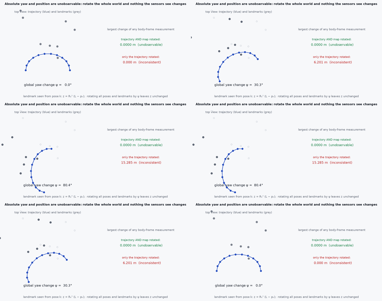
Engineering intuition
Shift the whole world a metre east and rotate it about the vertical: every image of the environment and every IMU measurement (relative to gravity) is unchanged. Position and yaw are therefore unobservable in VIO: four degrees of freedom, the “gauge”. The true uncertainty in those directions grows with time (drift). A filter whose linearisation points happen to depend on its current estimate can, through numerical accident, appear to learn about yaw from a measurement that contains none: its covariance in yaw shrinks when it should not. That is inconsistency, and the cure is to build the Jacobians so the unobservable directions stay in their null space.
Mathematical formulation
For the linear system, the observability matrix and its rank test:
Example: position–velocity with an accelerometer bias (state [, , ]); acceleration measured as a . With only a velocity or position measurement the bias is observable if the vehicle accelerates (the bias then changes the prediction), but with no measurement of position or velocity the whole state is unobservable. For the nonlinear VIO case, observability is analysed with Lie derivatives (Hesch et al., Kelly and Sukhatme): the result is four unobservable directions (3 translation, 1 yaw), plus scale becoming unobservable in a monocular system without sufficient excitation.
Consistency requires that the filter’s linearised model have the same unobservable subspace as the true nonlinear system. Observability-constrained EKF (OC-EKF) and first-estimate Jacobians enforce this: they choose the linearisation points so that contains the true gauge directions.
- observability matrix (linear case) or observability Gramian.
- directions that cannot be inferred from the data.
Architecture and data flow
The practical consequence for system design: provide a measurement that observes what you need. GNSS observes position and (via motion) heading, a magnetometer observes yaw, a map or loop closure observes the gauge directions in a drifting VIO. A navigation manager should know which states are observable in each mode and report a growing covariance in the others (lesson M2-T16).
Real-world UAV applications
- Deciding whether VIO needs a heading source for long flights.
- Checking that a filter keeps yaw uncertainty growing without GNSS.
- Choosing manoeuvres that excite scale or bias for calibration.
- Explaining overconfident covariance in a research estimator.
Implementation example
This runs as shown: observability ranks for a 1-D inertial navigation model with accelerometer bias and for a planar vehicle with yaw, and the observability Gramian eigenvalues for a constant-heading case.
import numpy as np

def obs_matrix(F, H, n):
    blocks, M = [], np.eye(n)
    for _ in range(n): blocks.append(H @ M); M = F @ M
    return np.vstack(blocks)
rank = lambda O: np.linalg.matrix_rank(O, tol=1e-9)

dt = 0.1
# 1-D inertial navigation: state [p, v, b_a]; the accelerometer measures a + b_a, which we treat as a known input u (so the bias drives velocity)
F = np.array([[1, dt, 0], [0, 1, -dt], [0, 0, 1.0]])
assert rank(obs_matrix(F, np.array([[1.0, 0, 0]]), 3)) == 3         # position measurements make velocity and bias observable
assert rank(obs_matrix(F, np.array([[0, 1.0, 0]]), 3)) == 2         # velocity alone: absolute position stays unobservable
assert rank(obs_matrix(F, np.array([[0, 0, 0.0]]), 3)) == 0         # no measurement: nothing is observable

# planar vehicle, state [x, y, yaw], heading-referenced position increments only observe relative motion
F3 = np.eye(3); H_rel = np.array([[0.0, 0, 0]])
assert rank(obs_matrix(F3, H_rel, 3)) == 0                          # odometry alone: no absolute pose is observable (gauge)
H_pos = np.array([[1.0, 0, 0], [0, 1.0, 0]])
assert rank(obs_matrix(F3, H_pos, 3)) == 2                          # absolute position observes x and y, yaw remains unobservable
H_all = np.vstack([H_pos, [0, 0, 1.0]])
assert rank(obs_matrix(F3, H_all, 3)) == 3                          # adding a heading source (magnetometer, GNSS course) observes yaw

# observability Gramian eigenvalues: the unobservable direction has (numerically) zero information
G = sum(np.linalg.matrix_power(F3.T, k) @ H_pos.T @ H_pos @ np.linalg.matrix_power(F3, k) for k in range(10))
lam = np.linalg.eigvalsh(G); print("Gramian eigenvalues (x, y observed):", np.round(lam, 3))
assert lam[0] < 1e-12 and lam[-1] > 5Common engineering mistakes
Assuming a state is observable because it appears in the model
Rank-test it; yaw and absolute position are typical gauge directions.
Linearising at the current estimate in a way that breaks the null space
The filter learns spurious information; use first-estimate Jacobians or an OC formulation.
Inflating process noise to hide the symptom
Treats the effect, not the cause.
Expecting calibration states to converge without excitation
Extrinsics and scale need motion.
Ignoring that observability depends on motion
Straight constant-velocity flight can make states unobservable.
Failure modes
| Failure mode | How it shows up | Likely cause |
|---|---|---|
| Spurious yaw certainty | Yaw covariance shrinks without a heading measurement | Inconsistent linearisation |
| Scale drift | Monocular scale wanders in straight flight | No acceleration excitation |
| Calibration not converging | Extrinsic estimate stays at its initial value | No rotation excitation |
| Overconfident output | NEES high only in unobservable states | Gauge directions not respected |
Debugging approach
- Compute the rank and the null space of the observability matrix of your model.
- Run NEES on sub-blocks: position, yaw, biases separately (lesson M3-T15).
- Check that yaw variance grows monotonically without a heading source.
- Design excitation manoeuvres and check convergence of calibration states.
Practical exercises
- Compute the observability matrix of a 2-D constant-velocity model measuring position only.
- Show that adding a magnetometer makes yaw observable in the planar example.
- Explain why scale is unobservable for a monocular camera flying at constant velocity.
- Find the dimension of the unobservable subspace of VIO with unknown camera–IMU extrinsics (see the references).
Interview questions
Write an answer in your own words, then reveal the model answer. Nothing is sent anywhere.
Question 1
What are the unobservable directions of VIO?
Model answer
Global position (three) and yaw about gravity (one): shifting or rotating the world about the vertical changes no measurement; roll, pitch, scale and biases are observable with sufficient motion.
Question 2
Why do some filters become inconsistent in unobservable directions?
Model answer
Linearising at the current estimate can give the filter spurious information in those directions, shrinking its covariance when the truth is drift.
Question 3
How do you make yaw observable?
Model answer
Add a measurement that depends on it: magnetometer, GNSS course or position over a path, a map or loop closure.
References and further reading
Primary papers, official documentation and standards. Each claim above that is specific to a tool or version points here.
- J. A. Hesch, D. G. Kottas, S. L. Bowman, S. I. Roumeliotis, “Camera-IMU-based localization: observability analysis and consistency improvement”, IJRR, 2014
- J. Kelly, G. S. Sukhatme, “Visual-inertial sensor fusion: localization, mapping and sensor-to-sensor self-calibration”, IJRR, 2011
- . . Barfoot, State Estimation for Robotics, Cambridge University Press, 2017, chapter 3.
- . . Chen, Linear System Theory and Design, 3rd ed., Oxford University Press, 1999.