UAV Systems Engineering · Module 5
M5-T12: Kinodynamic planning
Geometric planners ignore how the vehicle moves. Kinodynamic planners plan positions and velocities together, so the result can actually be flown.
A path through free space is not a trajectory. A quadrotor cannot turn a right angle at speed: acceleration is bounded by thrust and tilt, and its rate by motor dynamics. Kinodynamic planning builds those limits into the search itself, so the plan is feasible by construction. It is an active research area, with several competing formulations.
Learning objectives
After this lesson, you should be able to:
- Explain why a geometric path may be dynamically infeasible and what kinodynamic planning changes.
- Describe motion-primitive search in a state space of position and velocity with bounded acceleration.
- State what differential flatness gives a quadrotor planner.
- Name the front-end/back-end structure and the role of a safe flight corridor.
Conceptual explanation
Research-level Kinodynamic planning is an active research topic. This lesson describes common formulations from the literature (for example Mellinger and Kumar 2011 for minimum-snap polynomial trajectories; Liu et al. 2017 for safe-flight-corridor planning; Zhou et al. 2019 for a robust quadrotor planner). It is not a settled single method, and published results depend on the maps and vehicles they used.
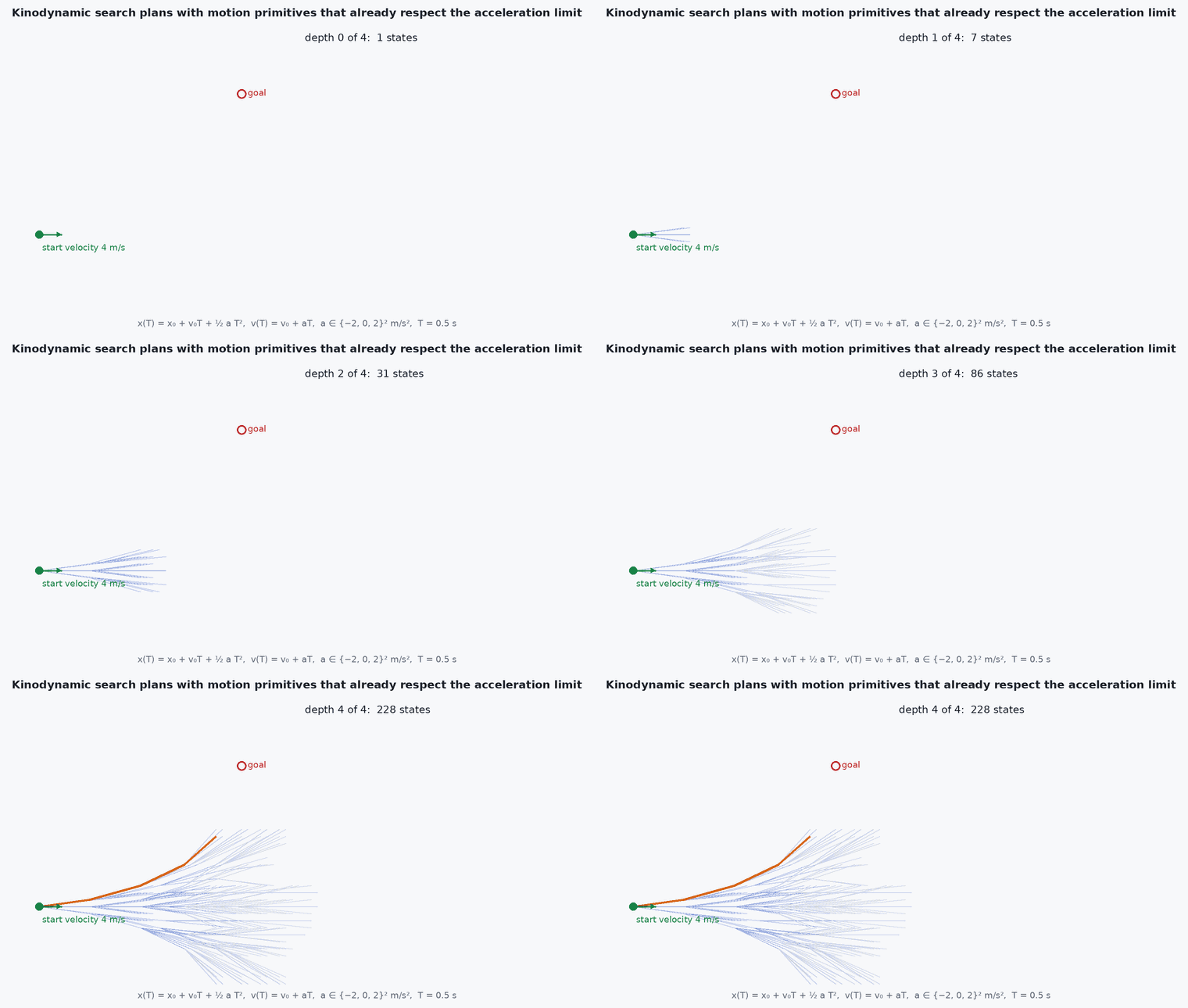
Kinodynamic means planning under kinematic and dynamic constraints. The state is no longer a position but position and velocity (and possibly acceleration), and the “edges” of the search are short trajectories produced by applying a bounded control (for example a constant acceleration) for a fixed time. Because those edges are executable, the whole plan is too.
Two properties make this practical for multirotors:
- Differential flatness: the full state and inputs of a quadrotor can be computed from the position and yaw trajectories and their derivatives (up to the fourth derivative of position, snap). Planning in the flat outputs reduces the problem to smooth curves in 3D.
- Polynomial trajectories have closed-form derivatives, so constraint checks and cost (for example the integral of squared snap) are cheap.
Engineering intuition
Think of driving a car: you cannot choose to be 5 m to the left instantly; you steer, and the lateral motion happens over seconds. A geometric planner draws the lane change as a kink; a kinodynamic planner plans the steering. For a quadrotor the equivalent is that horizontal acceleration requires tilt, and tilt takes time and thrust margin. A path with a corner at 8 m/s demands acceleration that does not exist, so the controller falls behind and the vehicle cuts the corner into whatever was there.
The planner’s dynamic model is a simplification: usually a triple integrator with bounds on velocity, acceleration and sometimes jerk. Anything it ignores (drag, wind, motor lag, controller tracking error) must be covered by margins, because feasibility on paper does not guarantee feasibility in the air.
Mathematical formulation
A common planning model is the triple integrator per axis with the jerk (or acceleration) as control: state , . For a motion primitive with constant jerk over time the end state is exact:
The minimum-snap trajectory through waypoints with polynomial segments minimises
For a fixed segment time allocation this is a quadratic program in the polynomial coefficients. Time allocation is the hard part: it is nonconvex, and common practice is heuristic (trapezoidal speed profile) followed by iteration. A safe flight corridor is a sequence of convex regions (polyhedra) covering the path; the back end then constrains the trajectory to the corridor with linear constraints.
Feasibility of the thrust: with total thrust acceleration vector a − ( the gravity vector), the required thrust magnitude is and the tilt satisfies for acceleration directed up, so a bound follows (about at tilt, ignoring vertical acceleration).
- , , a,
- position, velocity, acceleration, jerk (per axis).
- snap
- fourth derivative of position.
- maximum tilt angle allowed by thrust margin and control authority.
Architecture and data flow
Map (ESDF or occupancy) → front-end search from the current predicted state to a goal using bounded-acceleration primitives (or a kinodynamic RRT*) → path → safe flight corridor → back-end minimum-snap or similar optimisation with velocity, acceleration and clearance constraints → trajectory (position, velocity, acceleration, yaw as functions of time) → tracking controller. Replanning runs at a few Hz to tens of Hz from a state predicted forward by the planning latency. The localisation error and map delay set the clearance margin.
Real-world UAV applications
- High-speed flight through cluttered environments with onboard sensing.
- Aggressive but safe racing and agile manoeuvres (research prototypes).
- Replanning around dynamic obstacles.
- Energy- or time-optimal inspection trajectories.
Implementation example
This runs as shown. A forward search over constant-acceleration primitives in a 2D grid world for a point-mass with bounded acceleration and speed. It finds a path through a gap between two obstacles that respects the bounds, and the test verifies that every primitive respects the limits and that nothing intersects an obstacle (checked on a fine time sampling of each primitive). It is a teaching example, not a production planner.
import heapq, math, itertools
import numpy as np

a_max, v_max, T = 2.0, 3.0, 0.5
obst = [(8.0, 0.0, 12.0, 6.0), (8.0, 9.0, 12.0, 20.0)]         # axis-aligned boxes (xmin, ymin, xmax, ymax): a gap at y in (6, 9)
accs = [(ax, ay) for ax in (-a_max, 0.0, a_max) for ay in (-a_max, 0.0, a_max)]
def free(p):
    return all(not (b[0] - 0.5 <= p[0] <= b[2] + 0.5 and b[1] - 0.5 <= p[1] <= b[3] + 0.5) for b in obst) and -2 <= p[0] <= 20 and -2 <= p[1] <= 20
def step(s, a):
    p, v = np.array(s[:2]), np.array(s[2:]); pts = []
    for tt in np.linspace(0, T, 6)[1:]:
        pts.append(p + v * tt + 0.5 * np.array(a) * tt ** 2)
    v2 = v + np.array(a) * T
    return pts, np.concatenate([pts[-1], v2])
def key(s): return (round(s[0] / 0.5), round(s[1] / 0.5), round(s[2] / 0.5), round(s[3] / 0.5))
start = np.array([0.0, 7.5, 0.0, 0.0]); goal = np.array([18.0, 7.5])
tie = itertools.count(); openq = [(0.0, next(tie), start, 0.0)]; best = {key(start): 0.0}; parent = {}; prim = {}; found = None
while openq:
    f, _, s, g = heapq.heappop(openq)
    if np.linalg.norm(s[:2] - goal) < 1.0 and np.linalg.norm(s[2:]) < 1.0: found = s; break
    for a in accs:
        pts, s2 = step(s, a)
        if np.linalg.norm(s2[2:]) > v_max or not all(free(q) for q in pts): continue
        g2 = g + T + 0.05 * (a[0] ** 2 + a[1] ** 2) * T; k = key(s2)
        if g2 < best.get(k, 1e18):
            best[k] = g2; parent[k] = key(s); prim[k] = (a, pts)
            h = np.linalg.norm(s2[:2] - goal) / v_max
            heapq.heappush(openq, (g2 + h, next(tie), s2, g2))
assert found is not None
k = key(found); chain = []
while k in parent: chain.append(prim[k]); k = parent[k]
chain = chain[::-1]
ok = all(abs(a[0]) <= a_max and abs(a[1]) <= a_max and all(free(q) for q in pts) for a, pts in chain)
print(f"found: {len(chain)} primitives, duration {len(chain) * T:.1f} s, within bounds and obstacle-free: {ok}")
assert ok and len(chain) * T < 15Common engineering mistakes
Planning with an unrealistic dynamic model
Planned accelerations exceed what the vehicle delivers; leave margin for drag, wind and controller lag.
Ignoring planning latency
Plan from the current state, not the predicted state at the time the plan will start executing.
Treating polynomial smoothness as obstacle-safety
A smooth trajectory can bulge out of a corridor between waypoints; constrain it explicitly.
Time allocation by a single fixed speed
Tight turns need slower segments.
Over-tuning on one map
Planner parameters that work in one environment may fail in clutter with different density.
Failure modes
| Failure mode | How it shows up | Likely cause |
|---|---|---|
| Tracking error grows at corners | Vehicle drifts wide on turns | Planned acceleration or jerk beyond what the controller and actuators deliver |
| Plan intersects obstacles after smoothing | Collision on execution | Optimiser not constrained to the corridor |
| No plan found in a gap | Planner gives up in narrow passages | Primitive set or resolution too coarse for the gap |
| Flip-flopping between routes | Replans choose different passages repeatedly | No commitment to the previous solution |
Debugging approach
- Plot the planned and flown position, velocity and acceleration against time and compare the peaks to the bounds.
- Check the corridor and the trajectory together in the map viewer.
- Replay recorded maps offline through the planner and measure latency.
- Compare the commanded and measured tilt angles to see whether the thrust margin is used up.
Practical exercises
- Reduce to in the example and report the change in duration.
- Add a 3 s planning delay and show how planning from the current (instead of predicted) state causes a jump.
- Compute the maximum horizontal acceleration for a tilt limit.
- Fit a quintic polynomial between two states (position, velocity, acceleration) and check the acceleration bound.
Interview questions
Write an answer in your own words, then reveal the model answer. Nothing is sent anywhere.
Question 1
What is differential flatness and why does it help quadrotor planning?
Model answer
The state and inputs can be written as functions of flat outputs (position and yaw) and their derivatives, so planning smooth position and yaw curves automatically yields dynamically consistent attitude, rate and thrust commands.
Question 2
Why a front-end and a back-end?
Model answer
The front end solves the nonconvex topological problem (which way around obstacles) with search; the back end solves a smooth, often convex, optimisation inside the chosen corridor for comfort, speed and clearance.
Question 3
What can make a kinodynamically feasible plan infeasible in flight?
Model answer
Unmodelled drag and wind, controller tracking error, actuator limits and lag, and latency between planning and execution.
References and further reading
Primary papers, official documentation and standards. Each claim above that is specific to a tool or version points here.
- Mellinger, D. & Kumar, V. (2011). Minimum snap trajectory generation and control for quadrotors. ICRA
- Liu, S. et al. (2017). Planning dynamically feasible trajectories for quadrotors using safe flight corridors in 3-D complex environments. IEEE RA-L 2(3)
- Zhou, B., Gao, F., Wang, L., Liu, C. & Shen, S. (2019). Robust and efficient quadrotor trajectory generation for fast autonomous flight. IEEE RA-L 4(4)
- LaValle, S. M. Planning Algorithms (free online book)