UAV Systems Engineering · Module 5
M5-T11: A* and RRT path planning
A* gives the cheapest path on a grid; RRT gives a feasible path in spaces too large to grid. Know what each guarantees and what each costs.
Planning answers “how do I get from here to there without hitting anything”. Two families dominate: graph search such as A*, and random sampling such as RRT and its asymptotically optimal variant RRT*. They make different promises, and a UAV pipeline usually uses the path from one as the input to trajectory optimisation.
Learning objectives
After this lesson, you should be able to:
- Implement A* on an occupancy grid with an admissible heuristic and explain optimality.
- Describe how RRT and RRT* build a tree and what “probabilistically complete” and “asymptotically optimal” mean.
- Choose between search-based and sampling-based planning for a given map and dimension.
- Explain why a planner path must be smoothed and time-parameterised before flying.
Conceptual explanation
Established A* (Hart, Nilsson and Raphael, 1968) and RRT (LaValle, 1998) are classical. RRT* is from Karaman and Frazzoli (2011). Statements about guarantees assume the stated conditions (admissible heuristic; a static map; an unbounded sample count for asymptotic results).
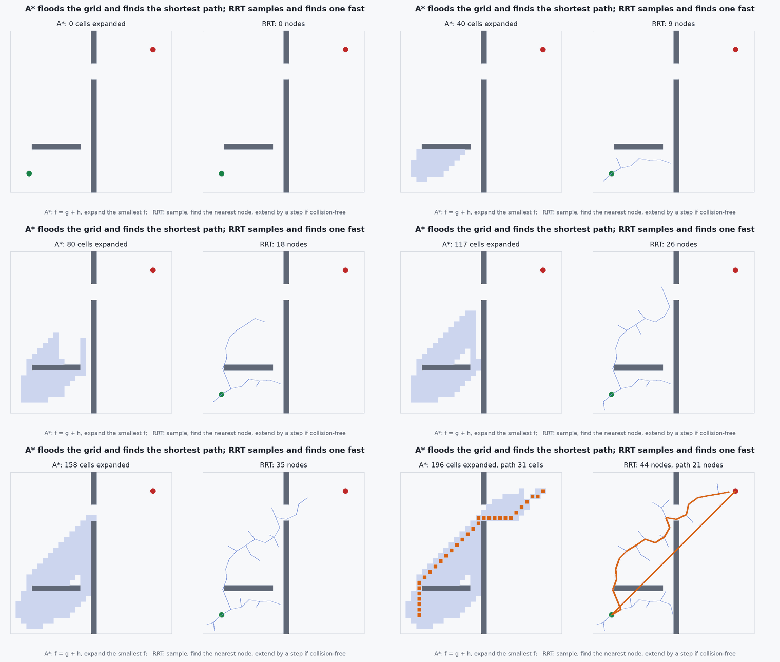
A* searches a graph by expanding the node with the smallest , where is the cost from the start and is a heuristic estimate of the cost to the goal. If never overestimates the true remaining cost (admissible) A* returns an optimal path on that graph; if it is also consistent, each node is expanded at most once.
RRT grows a tree from the start: sample a random state, find the nearest tree node, extend a short step toward the sample, keep the new node if the segment is collision-free. It is probabilistically complete: if a path exists the probability of finding one tends to 1 as samples increase. The path is typically jagged and non-optimal. RRT* rewires nearby nodes to reduce cost and is asymptotically optimal: the path cost converges to the optimum as samples tend to infinity.
Engineering intuition
A* is flood-filling with a compass: it explores outward but biases toward the goal, so open space is cheap. Its cost grows with the number of grid cells, so it suits 2D or 2.5D maps with metre-scale cells. In 3D with centimetre-scale cells the cell count explodes; the grid must be coarse, hierarchical or local.
RRT is throwing darts and connecting them: it does not care how big the space is, and handles high dimension (position plus velocity, or a manipulator’s joints) far better than grids do. The price is randomness: two runs differ, and the first path found is rarely good. For flight, that means a post-processing step (shortcutting, smoothing) and a time budget that cuts the search off.
Planners return paths in a map, and the map has errors. The planner should keep a safety margin from obstacles (inflate the map by the vehicle radius plus an allowance for localisation and tracking error) so that the path is flyable, not merely collision-free in an ideal world.
Mathematical formulation
On an 8-connected grid with cell size 1 the octile distance is an admissible, consistent heuristic; for Euclidean costs the straight-line distance is admissible:
RRT* chooses the best parent among nodes within a connection radius that shrinks slowly with samples; the published choice for asymptotic optimality is
Weighted A* uses with : it is faster but only -suboptimal (the path cost is at most times the optimum). Anytime variants start with a large and reduce it while time remains.
- (n)
- cost of the best known path from the start to .
- (n)
- heuristic estimate of the remaining cost.
- dimension of the planning space.
- inflation factor of weighted A*.
Architecture and data flow
Mapping (occupancy grid, ESDF or point cloud) → obstacle inflation → global planner (A* or RRT*) → path shortcutting → trajectory generation (see the trajectory-generation lesson) → tracking controller. For a UAV flying in unknown space the loop repeats: a local map is updated, collision of the current trajectory is checked, and the planner re-runs from the current state. The map’s age and the localisation drift both enter the safety margin.
Real-world UAV applications
- Global route planning in a known 2D or 2.5D map of a site.
- Local replanning around newly detected obstacles in a 3D occupancy map.
- Planning through cluttered environments such as warehouses and forests (sampling-based planning with a short time budget).
- Coverage and inspection path planning.
Implementation example
This runs as shown. A* on a 40 × 40 occupancy grid with a wall and a gap, 8-connected moves, octile heuristic. The test confirms that the path is collision-free and that its cost matches an independent Dijkstra search (A* with ), which verifies optimality of the admissible heuristic on this map.
import heapq, math

N = 40
blocked = {(20, y) for y in range(N) if y != 28}               # a wall at x = 20 with a gap at y = 28
blocked |= {(x, 10) for x in range(5, 18)}                      # a shorter wall
def neighbours(c):
    for dx in (-1, 0, 1):
        for dy in (-1, 0, 1):
            if (dx or dy):
                n = (c[0] + dx, c[1] + dy)
                if 0 <= n[0] < N and 0 <= n[1] < N and n not in blocked:
                    if dx and dy and ((c[0] + dx, c[1]) in blocked or (c[0], c[1] + dy) in blocked): continue   # no corner cutting
                    yield n, math.hypot(dx, dy)
def octile(a, b):
    dx, dy = abs(a[0] - b[0]), abs(a[1] - b[1]); return (math.sqrt(2) - 1) * min(dx, dy) + max(dx, dy)
def search(start, goal, use_h=True):
    openq = [(0.0, start)]; g = {start: 0.0}; parent = {}; expanded = 0
    while openq:
        f, c = heapq.heappop(openq)
        if f > g[c] + (octile(c, goal) if use_h else 0.0) + 1e-9: continue           # stale entry
        expanded += 1
        if c == goal:
            path = [c]
            while c in parent: c = parent[c]; path.append(c)
            return path[::-1], g[goal], expanded
        for n, w in neighbours(c):
            if g[c] + w < g.get(n, 1e18):
                g[n] = g[c] + w; parent[n] = c
                heapq.heappush(openq, (g[n] + (octile(n, goal) if use_h else 0.0), n))
    return None, None, expanded
start, goal = (2, 2), (37, 37)
path, cost, ex_a = search(start, goal, True)
path0, cost0, ex_d = search(start, goal, False)
print(f"A*: cost {cost:.2f}, {ex_a} expansions   Dijkstra: cost {cost0:.2f}, {ex_d} expansions")
assert all(c not in blocked for c in path) and abs(cost - cost0) < 1e-9 and ex_a < ex_dFor an RRT*, use a tested library rather than writing your own: the Open Motion Planning Library (OMPL) provides RRT, RRT*, Informed RRT* and many others with a common interface.
Common engineering mistakes
Inadmissible heuristic
Overestimating the remaining cost (for example a heuristic in different units from the edge cost) silently gives non-optimal paths.
Planning without obstacle inflation
The path grazes obstacles that the vehicle cannot clear once tracking error is included.
Flying the raw RRT path
It is jagged and costly; prune and smooth it first.
Ignoring replanning latency
The vehicle flies 1 m/s × 0.5 s = 0.5 m blind while the planner runs: plan from the predicted future state.
Mistaking probabilistic completeness for a time bound
It says nothing about how long the planner takes; always set a time budget and a fallback.
Failure modes
| Failure mode | How it shows up | Likely cause |
|---|---|---|
| No path found though one exists | Planner fails in narrow gaps | Inflation too large, resolution too coarse, too few samples |
| Path through an obstacle | Collision on execution | Map stale or inflation too small; collision test only at nodes rather than along segments |
| Oscillating replans | The path flips between two homotopies | No hysteresis or cost-to-commit on the current plan |
| Planner too slow | Vehicle stops and waits | Grid too fine; use a local window, weighted A*, or a time-limited anytime planner |
Debugging approach
- Visualise the map, inflated map, expanded nodes and path together.
- Test the planner on a map where the optimal path is known by hand.
- Compare with Dijkstra to verify optimality of A* implementations.
- Check segment (not only node) collision tests and the frame of the map against the vehicle pose.
Practical exercises
- Replace the octile heuristic with a heuristic multiplied by 3 and report cost and expansions (weighted A*).
- Add a cost layer that penalises cells within 2 cells of an obstacle and observe the path move away from walls.
- Implement an RRT in 2D with a 0.5 step and compare the first path found to the A* path.
- Inflate the map by the vehicle radius and show a gap that becomes impassable.
Interview questions
Write an answer in your own words, then reveal the model answer. Nothing is sent anywhere.
Question 1
What makes a heuristic admissible and why does it matter?
Model answer
It never overestimates the true remaining cost. With an admissible heuristic A* is guaranteed to return an optimal path on the graph; an inadmissible one can return suboptimal paths faster.
Question 2
What does probabilistically complete mean for RRT?
Model answer
If a solution exists the probability that the planner finds one approaches 1 as the number of samples grows. It gives no bound on time and no guarantee on path quality.
Question 3
Why is a planned path not directly flyable?
Model answer
It is geometric: it has corners and no timing. The vehicle has bounded acceleration and jerk, so the path must be smoothed and time-parameterised into a dynamically feasible trajectory.
References and further reading
Primary papers, official documentation and standards. Each claim above that is specific to a tool or version points here.
- Hart, P. E., Nilsson, N. J. & Raphael, B. (1968). A formal basis for the heuristic determination of minimum cost paths. IEEE Trans. Systems Science and Cybernetics
- Karaman, S. & Frazzoli, E. (2011). Sampling-based algorithms for optimal motion planning. IJRR 30(7)
- OMPL: the Open Motion Planning Library
- LaValle, S. M. Planning Algorithms (free online book)