UAV Systems Engineering · Module 5
M5-T13: Obstacle avoidance
Avoidance is a safety function: it needs a stopping-distance argument, a layered design and honest assumptions about sensor range and latency.
Planning avoids obstacles that are in the map; avoidance handles the ones that are not, or have moved, or appeared too late. The central design question is physical: can the vehicle stop or turn in the distance and time its sensors give it? Algorithms are secondary to that arithmetic.
Learning objectives
After this lesson, you should be able to:
- Compute the stopping distance of a UAV from speed, deceleration, sensing latency and range.
- Explain potential fields, velocity obstacles and control barrier functions and their weaknesses.
- Design a layered avoidance architecture with a last-resort stop.
- State what sensing range and field of view are required for a given speed.
Conceptual explanation
Established Potential fields (Khatib 1986), velocity obstacles (Fiorini and Shiller 1998) and control barrier functions (Ames et al. 2017) are published methods. How much speed a particular vehicle can safely fly with a particular sensor is an engineering measurement, not a property of the method.
Three families of reactive methods are common:
- Potential fields: the goal attracts and obstacles repel, and the vehicle follows the gradient. Simple and fast, but prone to local minima (the vehicle stalls between obstacles) and oscillation in narrow gaps.
- Velocity obstacles (VO): the set of relative velocities that lead to collision within a time horizon is excluded; the vehicle picks the allowed velocity closest to the desired one. Popular for moving obstacles and multi-agent avoidance.
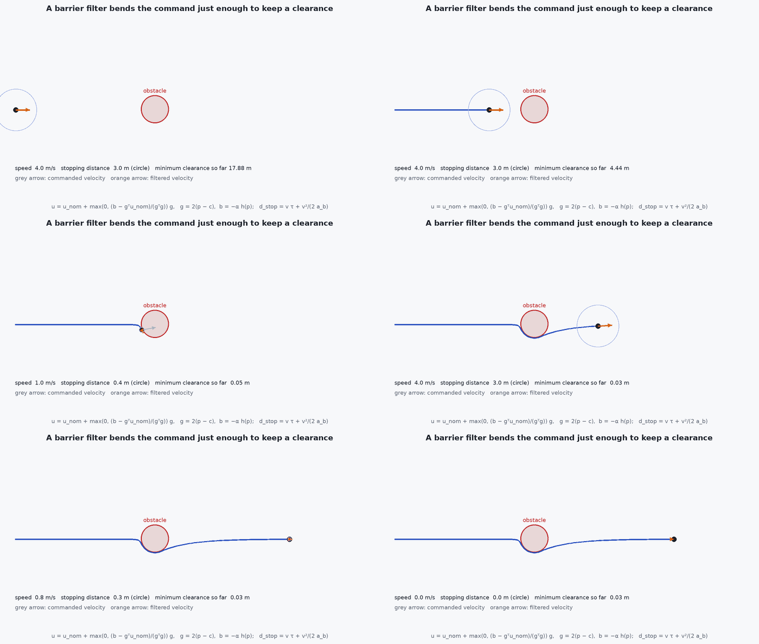
- Control barrier functions (CBF): a safety constraint is enforced by a small quadratic program that minimally modifies the nominal command so that never becomes negative. It provides a formal guarantee for the model and the sensing assumptions.
Engineering intuition
Avoidance is a race between how far you can see and how far you need to stop. A vehicle flying at 8 m/s with deceleration needs 8 m to stop even before accounting for any delay. A depth camera with a usable range of 5 m is therefore a hard limit: the vehicle cannot safely fly that fast in unknown space, whatever the algorithm. The safe speed follows from the sensing and braking physics.
The second intuition is that avoidance must run on a short cycle and use fresh data. A 200 ms-old depth frame at 5 m/s means the obstacle is already 1 m closer than the map shows. Latency is part of the stopping distance.
Mathematical formulation
Stopping distance for a vehicle at speed , constant braking deceleration and total sensing-to-actuation latency :
For safety the detection range must exceed plus a margin for localisation, mapping and tracking error: . Solving for the maximum speed:
The potential field force is for obstacle distance < ρ₀ (Khatib’s form). The CBF condition for ḣ = ∇h·(f + g u) is
with a design constant. For a sphere obstacle of radius around and a velocity-controlled point, and the constraint is linear in the commanded velocity, so the QP has a closed-form solution for one obstacle.
- ,
- speed and braking deceleration achievable in the worst direction and condition.
- latency from sensing to actuation: perception, planning, communication, actuator lag.
- ,
- reliable detection range and safety margin.
- (x)
- safety function: inside the safe set.
Architecture and data flow
Depth camera or lidar → local obstacle map (for example a voxel grid or an ESDF updated each frame) → planner re-checks the current trajectory for collision → if blocked, replan; independently, the reactive filter takes the commanded velocity and the nearest-obstacle geometry and outputs a safe velocity → position controller. A last-resort monitor reads the minimum range directly from the sensor and commands brake or hover if it falls below a hard threshold. All stages carry timestamps so that latency can be measured and added to .
Real-world UAV applications
- Collision avoidance in unknown environments with onboard depth sensing.
- Moving obstacle avoidance, including other aircraft in cooperative settings.
- Landing-zone clearance monitoring.
- Geofence-style soft boundaries implemented as barrier functions.
Implementation example
This runs as shown. A control-barrier-function velocity filter for a point vehicle with velocity control and a circular obstacle (radius 2 m). The vehicle tries to fly straight through the obstacle; the filter minimally modifies the velocity so that the distance never falls below the radius. The test checks the clearance and that, with no obstacle nearby, the command passes through unchanged. The numbers for stopping distance are also computed.
import numpy as np

def cbf_filter(p, u_nom, c, r, alpha):
    # h = ||p-c||^2 - r^2 ;  dh = 2 (p-c)^T u ;  require dh + alpha h >= 0  (a half-space constraint on u)
    g = 2.0 * (p - c); b = -alpha * (np.dot(p - c, p - c) - r ** 2)
    if g @ u_nom >= b: return u_nom                       # nominal command already satisfies the constraint
    return u_nom + (b - g @ u_nom) / (g @ g) * g          # projection onto the half-space (closed-form QP)

c, r, alpha, dt = np.array([20.0, 0.1]), 2.0, 1.5, 0.02
p = np.array([0.0, 0.0]); goal = np.array([40.0, 0.0]); clear = 1e9; passed_through = None
for k in range(int(30 / dt)):
    u_nom = np.clip(1.0 * (goal - p), -4.0, 4.0)
    u = cbf_filter(p, u_nom, c, r, alpha)
    if k == 0: passed_through = np.allclose(u, u_nom)
    p = p + u * dt; clear = min(clear, np.linalg.norm(p - c) - r)
print(f"minimum clearance to the obstacle surface: {clear:.3f} m, reached x = {p[0]:.1f}")
v, ab, tau = 8.0, 4.0, 0.25
print(f"stopping distance at {v} m/s, {ab} m/s^2, {tau} s latency: {v * tau + v ** 2 / (2 * ab):.1f} m")
assert clear > -1e-3 and passed_through and p[0] > 30
vmax = ab * (-tau + np.sqrt(tau ** 2 + 2 * (6.0 - 1.0) / ab)); print(f"max speed for R = 6 m, margin 1 m: {vmax:.2f} m/s")
assert abs(vmax * tau + vmax ** 2 / (2 * ab) - 5.0) < 1e-9Common engineering mistakes
Ignoring latency in the stopping distance
At 8 m/s a 250 ms delay is 2 m of travel before braking starts.
Assuming the sensor sees everything
Thin wires, glass, water, sun glare and low-texture walls defeat depth cameras and some lidars.
Trusting a potential field in clutter
Local minima make the vehicle stall or oscillate between obstacles.
No independent last-resort layer
If the planner fails or is slow, nothing stops the vehicle.
Barrier guarantee beyond its assumptions
A CBF is only as safe as the model, the obstacle position estimate and the actuator limits it assumes.
Failure modes
| Failure mode | How it shows up | Likely cause |
|---|---|---|
| Vehicle stalls between obstacles | Hover with no progress | Local minimum of a potential field or a conflict between layers |
| Late detection | Brakes too late, hits at low speed | Range or field of view below the stopping distance; stale data |
| Oscillation near an obstacle | Side-to-side chatter | High gain on repulsion, noisy range, no hysteresis |
| Missed obstacle class | Collides with thin or transparent objects | Sensor limitation not covered by the operating limits |
Debugging approach
- Log the minimum range, the commanded and filtered velocity, and the time of each frame used.
- Test the stopping distance in flight at increasing speeds against a soft obstacle or a marked line.
- Replay recorded sensor data into the avoidance layer offline.
- Characterise sensor failures: reflective, thin, dark and glass obstacles, and sunlight.
Practical exercises
- Compute the maximum safe speed for a 4 m reliable depth range, 0.2 s latency, deceleration and 0.5 m margin.
- Add a second obstacle and compute the constraint for each; use the more restrictive one or solve the small QP.
- Make the obstacle move at 1 m/s and show the clearance with and without a velocity-aware term.
- Design test cases for glass, wire and dark-surface obstacles.
Interview questions
Write an answer in your own words, then reveal the model answer. Nothing is sent anywhere.
Question 1
How do you decide the maximum safe speed for obstacle avoidance?
Model answer
From stopping distance: speed times total latency plus /(2a_b), which must be below the reliable detection range minus a margin. The sensor range, latency and braking capability set the speed, not the algorithm.
Question 2
What are the weaknesses of potential fields?
Model answer
Local minima, oscillation in narrow passages, and no formal guarantee. They are cheap and reactive but need a higher layer to avoid trapping.
Question 3
What does a control barrier function guarantee?
Model answer
For the assumed dynamics, obstacle estimate and actuation limits, the state stays in the safe set. Model error, sensing error and saturation can break the guarantee.
References and further reading
Primary papers, official documentation and standards. Each claim above that is specific to a tool or version points here.
- Khatib, O. (1986). Real-time obstacle avoidance for manipulators and mobile robots. IJRR 5(1)
- Fiorini, P. & Shiller, Z. (1998). Motion planning in dynamic environments using velocity obstacles. IJRR 17(7)
- Ames, A. D. et al. (2017). Control barrier function based quadratic programs for safety critical systems. IEEE TAC 62(8)
- PX4: Collision prevention