UAV Systems Engineering · Module 2
M2-T13: LiDAR-aided navigation
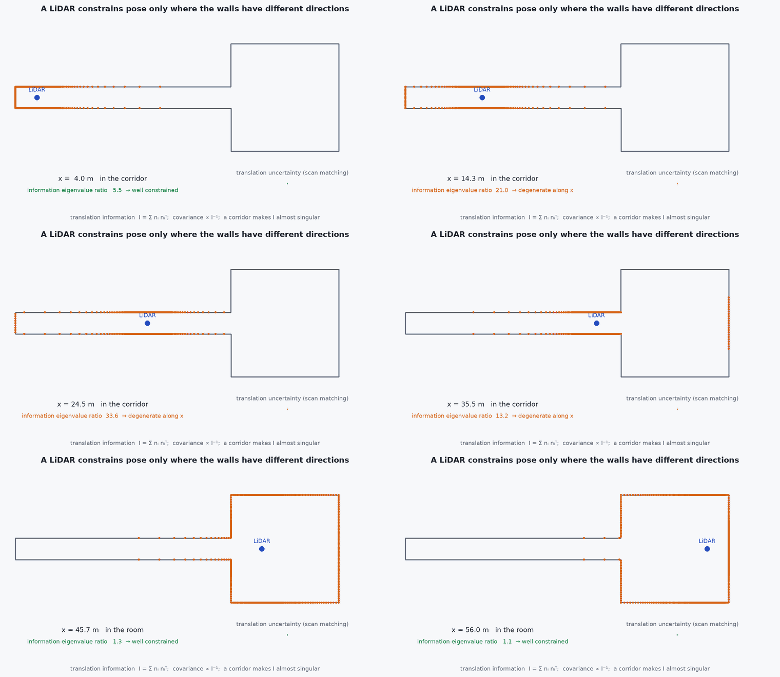
A LiDAR constrains pose only along directions in which the surfaces it sees change: in a long corridor it cannot tell you how far along you are.
LiDAR gives direct metric geometry independent of lighting, which is why it anchors many GNSS-denied UAV systems. Its weakness is geometric: some scenes do not constrain some directions. This lesson shows how to see that in the maths, and detect it at run time.
Learning objectives
After this lesson, you should be able to:
- Explain how a range scan constrains the vehicle pose through surface geometry.
- Write the point-to-plane residual and the information (Hessian) matrix it produces.
- Detect degenerate directions from the eigenvalues of the information matrix.
- List LiDAR failure modes: degeneracy, dust, rain, glass, vibration and motion distortion.
Conceptual explanation
A scanning LiDAR measures ranges along known beam directions, giving a point cloud in the sensor frame. Navigation uses it by registering the current scan to a reference (the previous scan or a map): the pose that best aligns the points to the surfaces. Each point on a planar surface constrains the pose only along that surface’s normal; the set of normals in the scene determines which directions are constrained.
Engineering intuition
Stand in a long straight featureless corridor with a LiDAR: the two walls and the floor and ceiling tell you exactly where you are across and above, but nothing tells you where you are along the corridor. Every candidate position along the axis sees the same scan. The same happens in an open field (flat ground constrains only height, roll and pitch) and next to a single wall. A registration algorithm in such a scene returns a confident-looking answer along the unconstrained direction that is simply the initial guess (or noise): it must be flagged, and a different sensor must constrain that direction.
Mathematical formulation
For a point (sensor frame), a pose (, ) and the plane through the map with unit normal and offset , the point-to-plane residual and its Jacobian for a small pose update are:
The information matrix and its eigen-decomposition give the constraint strength per direction:
The covariance of the registration is : a near-zero eigenvalue is an enormous variance in that direction, which an honest estimator must reflect (lesson M3-T12). The translational block alone is a 3×3 matrix : a corridor has normals in only two directions, so one eigenvalue is zero.
- unit normal of the plane at point .
- range noise of the sensor.
- threshold chosen from the required accuracy and .
Architecture and data flow
Scan with per-point time → IMU deskew (lesson M3-T10) → registration to the local map (lesson M2-T14, M4-T8) → pose, covariance and an explicit degeneracy flag (which directions are unconstrained) → estimator, which inflates the covariance in those directions or ignores them (as in degeneracy-aware LIO systems), and the navigation monitor (lesson M2-T16).
Real-world UAV applications
- GNSS-denied flight in warehouses, tunnels and under bridges.
- Detecting when to trust LiDAR odometry and when to lean on vision.
- Mapping and localisation (Capstone 2).
- Choosing a LiDAR with a wider field of view to see more normals.
Implementation example
This runs as shown: the translational information matrix for a room, a corridor and an open field; the corridor and field have rank deficiency the eigenvalues expose.
import numpy as np
rng = np.random.default_rng(0)

def scene_normals(kind, n=600):
    if kind == "room":     axes = np.eye(3)                                    # walls, floor, ceiling in all three directions
    elif kind == "corridor": axes = np.array([[0, 1, 0], [0, 0, 1]], float)     # side walls and floor/ceiling: nothing normal to the corridor axis (x)
    else:                  axes = np.array([[0, 0, 1]], float)                  # open field: flat ground only
    k = rng.integers(0, len(axes), n); nvec = axes[k] + 0.02 * rng.standard_normal((n, 3))      # a little roughness
    return nvec / np.linalg.norm(nvec, axis=1, keepdims=True)

def translation_information(normals, sigma=0.03): return normals.T @ normals / sigma ** 2

for kind in ("room", "corridor", "field"):
    lam = np.sort(np.linalg.eigvalsh(translation_information(scene_normals(kind))))[::-1]
    constrained = int(np.sum(lam > 1e-2 * lam[0]))
    sigma_axes = np.where(lam > 1e-2 * lam[0], 1 / np.sqrt(np.maximum(lam, 1e-12)), np.inf)
    print(f"{kind:9s} eigenvalues {np.round(lam, 0)} -> constrained directions: {constrained}")
    assert constrained == {"room": 3, "corridor": 2, "field": 1}[kind]
# the covariance along the weak direction is huge
lam = np.sort(np.linalg.eigvalsh(translation_information(scene_normals("corridor"))))
assert 1 / np.sqrt(max(lam[0], 1e-12)) > 10 / np.sqrt(lam[-1]) # at least ten times more uncertain along the weak directionCommon engineering mistakes
Reporting a covariance from the optimiser without a degeneracy check
In a corridor the registration returns an answer along the axis with false confidence.
Assuming more points means more constraint
Constraint comes from normal diversity, not point count.
Ignoring dust, rain and fog returns
They create false surfaces near the sensor; filter by range and intensity.
Mounting without a clear field of view
The airframe and propellers appear as obstacles in the scan.
Not deskewing
At UAV speeds a scan is distorted by motion (lessons M3-T10, M4-T8).
Failure modes
| Failure mode | How it shows up | Likely cause |
|---|---|---|
| Corridor drift | Drift along the corridor axis with small reported covariance | Degenerate geometry |
| Glass and mirrors | Missing or phantom surfaces | Specular surfaces defeat LiDAR returns |
| Dust and rain | False returns, odometry jitter | Particles near the sensor |
| Vibration blur | Smeared surfaces | Unsynchronised IMU or motion not deskewed |
Debugging approach
- Plot the eigenvalues of the registration information over time and mark corridors.
- View the accumulated map for double surfaces.
- Compare drift along and across a corridor.
- Test with a deliberate corridor and a flat field segment.
Practical exercises
- Prove that has rank equal to the dimension spanned by the normals.
- Choose for a 0.05 m accuracy requirement and .
- Describe which other sensor constrains the along-corridor direction and how.
- Count the constrained directions for a scene with a single wall.
Interview questions
Write an answer in your own words, then reveal the model answer. Nothing is sent anywhere.
Question 1
Why can LiDAR odometry drift in a long corridor?
Model answer
The surface normals span only two directions, so motion along the corridor axis changes no residual: the scan registration does not constrain it.
Question 2
How do you detect degeneracy at run time?
Model answer
From the eigenvalues of the information matrix (or the registration Hessian): a small eigenvalue marks an unconstrained direction.
Question 3
What should the estimator do with a degenerate direction?
Model answer
Treat it as unobserved: inflate its covariance or exclude the update, and rely on another sensor for it.
References and further reading
Primary papers, official documentation and standards. Each claim above that is specific to a tool or version points here.