UAV Systems Engineering · Module 2

M2-T14: LiDAR odometry

Align this scan to the last one, and the transform between them is the vehicle’s motion: ICP is the iteration that finds it.

Lesson 14 of 16
UAV Navigation and GNSS-Denied Operations
Established engineering
About 5 minutes to read

LiDAR odometry integrates the transforms between consecutive scans, or between a scan and a local map. The core algorithm, iterative closest point, is old, simple and sensitive to initialisation: understanding where it converges and where it does not is most of the engineering.

Learning objectives

After this lesson, you should be able to:

Describe the ICP iteration: correspondence, alignment, update.
Contrast point-to-point and point-to-plane error metrics and scan-to-scan with scan-to-map registration.
Explain the convergence basin and the role of the IMU initial guess.
Implement 2-D ICP and test it against a known transform.

Conceptual explanation

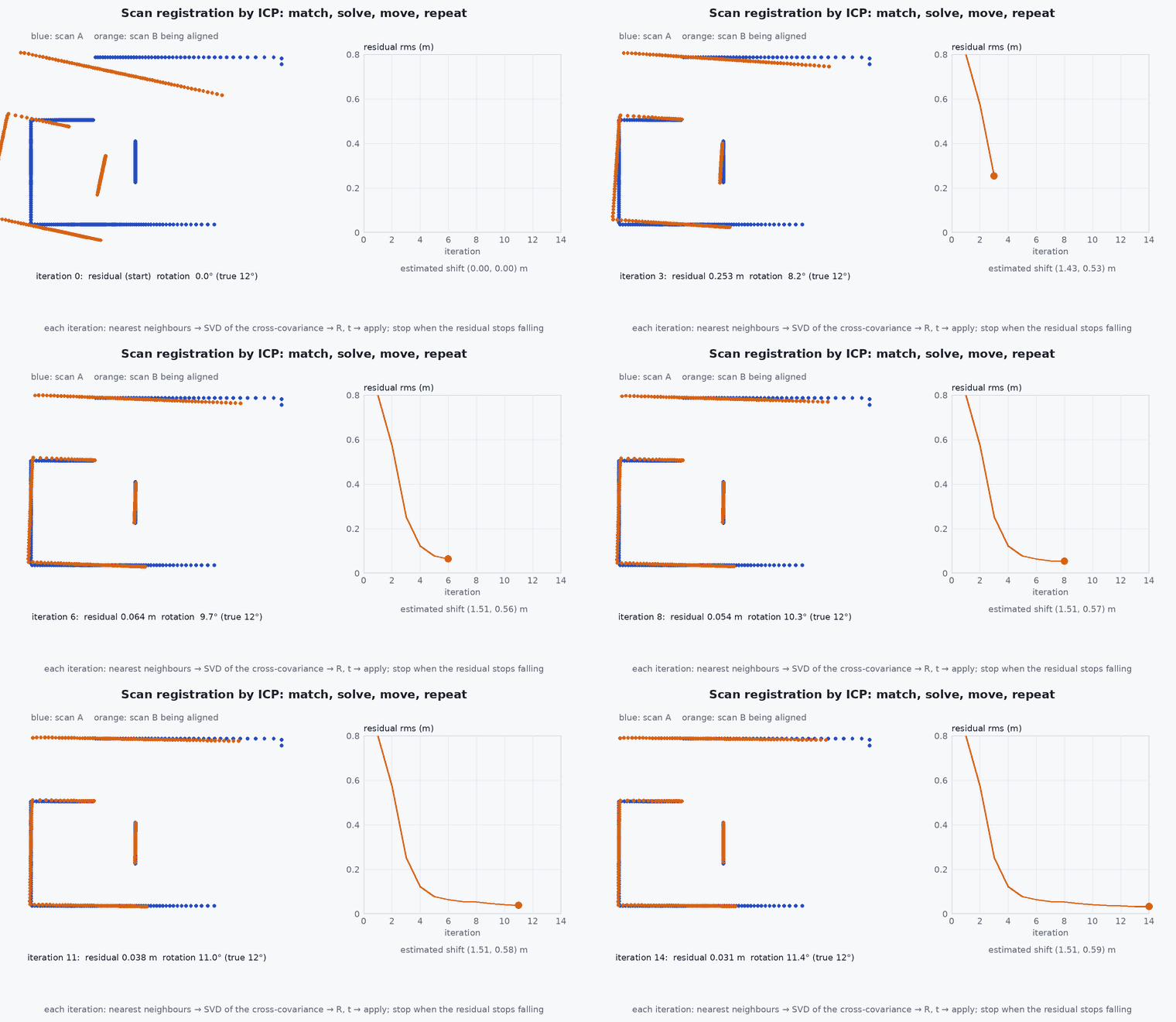
Iterative closest point (ICP) aligns a source cloud $S$ to a target cloud $T$ by repeating: (1) for each source point find the nearest target point; (2) compute the rigid transform that best aligns the matched pairs; (3) apply it and repeat until the change is small. Scan-to-scan registration is cheap but accumulates drift quickly; scan-to-map registration against an accumulated local map drifts more slowly because errors are not compounded frame by frame.

The ICP iteration.

Animation of iterative closest point registration of two LiDAR scans of the same room taken from poses 1.5 metres and 12 degrees apart. The second scan is moved towards the first over ten iterations; each iteration pairs every point with its nearest neighbour, solves the best rigid transform by singular value decomposition and applies it. The residual falls from about half a metre to a few centimetres and the estimated pose converges to the true relative pose. — ICP alternates nearest-neighbour matching with a closed-form rigid-transform solution. It converges to the true motion when the start is close enough and the scene has enough structure (previous lesson); the residual and the number of iterations show convergence. Computed in 2D on ray-cast scans. (Looping, about 6 seconds; drawn and computed for this course with illustrative values.)

Engineering intuition

ICP is gradient-like descent on a cost with many local minima: with a poor starting guess, nearest-neighbour matches are wrong and the alignment settles into a wrong minimum, usually a slightly shifted copy of the structure. Hence the IMU’s role: it predicts the inter-scan motion accurately over 0.1 s, so ICP starts inside the basin of convergence. And a moving sensor distorts each scan during acquisition: the IMU motion is also used to deskew the points before registration.

Mathematical formulation

For matched pairs $(p_{i},\,q_{i})$ the point-to-point step minimises $\sum \Vert R\,p_{i}+t-q_{i}\Vert ^{2}$ , solved in closed form by SVD of the cross-covariance (as in lesson M2-T12):

Point-to-point alignment step

\mathbf H = \sum_i(\mathbf p_i - \bar{\mathbf p})(\mathbf q_i - \bar{\mathbf q})^{\top} = \mathbf U\boldsymbol\Sigma\mathbf V^{\top}

\mathbf R = \mathbf V\operatorname{diag}\!\left(1,\dots,\det(\mathbf V\mathbf U^{\top})\right)\mathbf U^{\top}, \qquad \mathbf t = \bar{\mathbf q} - \mathbf R\,\bar{\mathbf p}

Point-to-plane minimises the distance to the target’s local tangent plane, which converges faster on structured scenes:

Point-to-plane objective

\min_{\mathbf R,\,\mathbf t}\ \sum_i\left[\mathbf n_i^{\top}(\mathbf R\mathbf p_i + \mathbf t - \mathbf q_i)\right]^{2}

Linearised in the small rotation, this is a 6×6 linear system per iteration.

$p_{i}$: source points (current scan).
$q_{i}$ , $n_{i}$: matched target points and their surface normals.
$R$ , $t$: rigid transform being estimated.

Robust variants weight or reject pairs by distance (trimmed ICP), and generalised ICP uses local covariances of both clouds. Nearest-neighbour search uses a k-d tree; FAST-LIO2’s ikd-Tree supports incremental updates (lesson M4-T8).

Architecture and data flow

IMU prediction gives the initial transform; deskewing corrects points to a common time; registration against the local map yields the pose update and an information matrix (lesson M2-T13); the new scan is added to the map and old points removed. The accumulated pose is the odometry output.

Real-world UAV applications

Odometry in LOAM, LIO-SAM and FAST-LIO2 variants.
Map-based localisation against a prior map (lesson M4-T13).
Loop-closure verification by registration (lesson M4-T11).
Sensor-to-sensor extrinsic refinement.

Implementation example

This runs as shown: a 2-D point-to-point ICP aligns a noisy scan of a structured room to the same room seen from a displaced pose, converging from a modest initial error and failing from a large one.

import numpy as np
rng = np.random.default_rng(0)

def room_scan(pose, n=360, noise=0.01):
    x, y, th = pose; pts = []
    walls = [((0, 1.0), 4.0), ((0, -1.0), 3.0), ((1.0, 0), 5.0), ((-1.0, 0), 5.0)]            # n.q = d
    for a in np.linspace(0, 2 * np.pi, n, endpoint=False):
        dw = np.array([np.cos(a + th), np.sin(a + th)]); best = 1e9
        for nv, d in walls:
            nv = np.array(nv); den = nv @ dw
            if den > 1e-6: lam = (d - nv @ np.array([x, y])) / den; best = min(best, lam) if lam > 0 else best
        pts.append(best * np.array([np.cos(a), np.sin(a)]) + noise * rng.standard_normal(2))      # point in the sensor frame
    return np.array(pts)

def best_transform(P, Q):
    Pc, Qc = P.mean(0), Q.mean(0); U, _, Vt = np.linalg.svd((P - Pc).T @ (Q - Qc))
    R = Vt.T @ np.diag([1, np.linalg.det(Vt.T @ U.T)]) @ U.T; return R, Qc - R @ Pc

def icp(src, tgt, iters=60, init=(np.eye(2), np.zeros(2))):
    R, t = init
    for _ in range(iters):
        moved = src @ R.T + t
        d2 = ((moved[:, None, :] - tgt[None, :, :]) ** 2).sum(-1); nn = tgt[d2.argmin(1)]           # nearest-neighbour correspondences
        dR, dt = best_transform(moved, nn); R, t = dR @ R, dR @ t + dt
    return R, t

move = np.array([0.30, -0.15, np.radians(8.0)])                                                      # true motion between the scans
A = room_scan((0.0, 0.0, 0.0)); B = room_scan(tuple(move))
c, s = np.cos(move[2]), np.sin(move[2]); R_true = np.array([[c, -s], [s, c]]); t_true = move[:2]
# B is expressed in the frame at the new pose: map B into A's frame with (R_true, t_true)
R, t = icp(B, A, init=(np.eye(2), np.zeros(2)))
err_t = np.linalg.norm(t - t_true); err_r = abs(np.arctan2(R[1, 0], R[0, 0]) - move[2])
print(f"from identity guess: translation error {err_t * 100:.1f} cm, rotation error {np.degrees(err_r):.2f} deg")
assert err_t < 0.05 and err_r < np.radians(1.0)
R2, t2 = icp(B, A, init=(np.array([[np.cos(2.5), -np.sin(2.5)], [np.sin(2.5), np.cos(2.5)]]), np.zeros(2)))      # a bad initial guess: 143 degrees off
print(f"from a bad guess: translation error {np.linalg.norm(t2 - t_true):.2f} m, rotation {np.degrees(np.arctan2(R2[1, 0], R2[0, 0])):.0f} deg (true 8)")
assert np.linalg.norm(t2 - t_true) > 3 * err_t                                                        # the basin of convergence is limited

2-D point-to-point ICP: converges from the identity guess and settles into a wrong, flipped alignment from a 143° guess.

Common engineering mistakes

Starting ICP from the identity at speed

Large inter-scan motion leaves the convergence basin; use the IMU prediction.

Scan-to-scan only

Drift accumulates quickly; register to a local map.

Not removing dynamic points

Moving objects pull the alignment.

Fixed correspondence threshold

Too tight misses, too loose admits outliers; use a decreasing or robust threshold.

Ignoring the computation budget

Map size drives nearest-neighbour cost (lesson M7-T3).

Failure modes

Failure modes, symptoms and causes
Failure mode	How it shows up	Likely cause
Wrong local minimum	Map shows doubled structure	Poor initial guess
Degenerate scene	Drift along an unconstrained direction	Corridor or open field
Moving objects	Pose pulled by a person or vehicle	No dynamic filtering
Slow processing	Latency grows with map size	Map not bounded

Debugging approach

Visualise the source and target after registration.
Plot the residual and inlier fraction against time.
Log the IMU prediction error: large errors mean the initial guess is the issue.
Check scan timestamps and deskewing.

Practical exercises

Implement the point-to-plane variant and compare the iterations to converge.
Find the largest initial rotation from which the example still converges.
Add a rejection of the 20% worst pairs and measure the effect with outliers.
Estimate the nearest-neighbour cost for a map of $10^{6}$ points with a k-d tree.

Interview questions

Write an answer in your own words, then reveal the model answer. Nothing is sent anywhere.

Question 1

What are the steps of ICP?

Model answer

Match each source point to its nearest target point, compute the rigid transform that best aligns the matches, apply it, and iterate until convergence.

Question 2

Why is the initial guess important?

Model answer

ICP is local: wrong correspondences from a poor start lead to a wrong minimum; the IMU gives an accurate initial motion estimate.

Question 3

Why prefer scan-to-map over scan-to-scan?

Model answer

Registering to an accumulated map reduces compounding drift because each scan is tied to a consistent reference rather than only the previous noisy one.

References and further reading

Primary papers, official documentation and standards. Each claim above that is specific to a tool or version points here.

What’s next

Mark this lesson

Saved in this browser and synced to your account when you are signed in.

Practice this lesson

M2-L5: Compare IMU-only, VIO and LiDAR odometry

Run the three estimators on one trajectory and compare error growth.

Next lesson

M2-T15: Radar-aided navigation

Describe how radar provides range, Doppler velocity and robustness to dust and darkness.