UAV Systems Engineering · Module 3
M3-T11: Multi-sensor fusion architectures
How you wire the filters decides whether information is counted once or twice, and whether one bad sensor can be isolated.
With several estimators (VIO, LIO, GNSS) the architecture question is unavoidable: one big filter, several small ones combined, or one optimisation over everything. Each answers the question of correlation and fault isolation differently.
Learning objectives
After this lesson, you should be able to:
- Compare centralised, federated and factor-graph fusion.
- Explain double counting when combining correlated estimates.
- Apply covariance intersection to fuse estimates with unknown correlation.
- Choose an architecture for a design with fault-isolation requirements.
Conceptual explanation
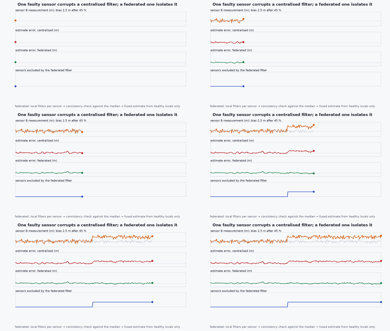
Centralised fusion feeds every raw measurement to one filter: optimal and consistent when modelled correctly, but one fault can contaminate everything and complexity grows. Federated (decentralised) fusion runs local filters per sensor group and combines their outputs; isolation is easy, but local estimates share the same IMU and process noise, so they are correlated. Factor-graph smoothing optimises over a window of states with factors from every sensor, handling asynchrony and delayed data well at higher compute.
| Architecture | Strength | Weakness | Typical use |
|---|---|---|---|
| Centralised EKF | consistent, simple to reason about | a bad sensor can corrupt the state; monolith | autopilot estimators (EKF2) |
| Federated | fault isolation, modular | correlated outputs, care to avoid double counting | redundant navigation with independent subsystems |
| Factor graph | handles delays, relinearisation, loop closure | compute, latency | VINS-Fusion, ORB-SLAM3, LIO-SAM |
Engineering intuition
Two navigation filters both using the same IMU have errors that are correlated through the IMU noise. Averaging their outputs as if independent halves the variance in the books but not in reality: the combined covariance is too small, the filter is overconfident. Covariance intersection (CI) gives a fused estimate that is consistent for any correlation, at the price of being more conservative than the optimal fusion when the estimates really are independent.
Mathematical formulation
Naive fusion of two independent estimates and in information form:
Covariance intersection for unknown correlation, with weight chosen to minimise, for example, the trace or determinant of :
CI is guaranteed consistent ( ≥ true error covariance) whatever the cross-correlation. When one estimate carries the other’s information already (a VIO built on the same IMU as the autopilot’s EKF), CI is the safe combination; for independent estimates it is conservative.
- weight of the first estimate (scalar), chosen by a one-dimensional search.
- covariance of estimate .
Architecture and data flow
In the reference architecture the IMU-driven fusion estimator on the companion combines VIO, LIO and GNSS (centralised or factor-graph), and its output enters PX4’s EKF2 as external odometry: EKF2 then holds a second estimator using the same IMU, a federated structure. Treat the external odometry covariance conservatively (inflate it) because EKF2’s own IMU propagation is correlated with it.
Real-world UAV applications
- Designing redundant navigation for fault isolation.
- Combining VIO from the companion with the autopilot’s estimate.
- Multi-vehicle cooperative localisation.
- Choosing between EKF and a factor graph for a research estimator.
Implementation example
This runs as shown: two estimates with correlated errors (shared process noise) are fused naively and with covariance intersection; the naive fusion is overconfident (NEES too high) and CI is consistent (NEES at most the expected value).
import numpy as np
rng = np.random.default_rng(0)
N = 20000
shared = rng.standard_normal((N, 2)) * 1.0                       # error component common to both estimates (e.g. from a shared IMU)
e1 = shared + 0.5 * rng.standard_normal((N, 2)); e2 = shared + 0.7 * rng.standard_normal((N, 2))
P1 = np.eye(2) * (1.0 + 0.25); P2 = np.eye(2) * (1.0 + 0.49)     # each estimate's true error covariance (shared + own)
true = np.zeros(2); x1, x2 = true + e1, true + e2

def fuse_naive(x1, x2, P1, P2):
    I1, I2 = np.linalg.inv(P1), np.linalg.inv(P2); P = np.linalg.inv(I1 + I2)
    return (P @ (I1 @ x1.T + I2 @ x2.T)).T, P
def fuse_ci(x1, x2, P1, P2):
    I1, I2 = np.linalg.inv(P1), np.linalg.inv(P2)
    w = min(np.linspace(0, 1, 101), key=lambda w: np.trace(np.linalg.inv(w * I1 + (1 - w) * I2)))   # minimise the trace of the fused covariance
    P = np.linalg.inv(w * I1 + (1 - w) * I2); return (P @ (w * I1 @ x1.T + (1 - w) * I2 @ x2.T)).T, P

def mean_nees(x, P): e = x - true; return np.mean(np.einsum('ij,jk,ik->i', e, np.linalg.inv(P), e))
xn, Pn = fuse_naive(x1, x2, P1, P2); xc, Pc = fuse_ci(x1, x2, P1, P2)
print(f"mean NEES (expected <= 2): naive {mean_nees(xn, Pn):.2f}, covariance intersection {mean_nees(xc, Pc):.2f}; fused std: naive {np.sqrt(Pn[0, 0]):.2f}, CI {np.sqrt(Pc[0, 0]):.2f}")
assert mean_nees(xn, Pn) > 2.5 and mean_nees(xc, Pc) <= 2.05                  # naive: overconfident; CI: consistent (conservative)
assert np.sqrt(Pc[0, 0]) > np.sqrt(Pn[0, 0]) # CI admits the shared error that the naive fusion hidesCommon engineering mistakes
Averaging correlated estimates as independent
The covariance shrinks too fast: overconfidence.
Feeding a filter’s output back into itself
Information is counted repeatedly (a loop).
Using one big filter without fault isolation
A single faulty sensor corrupts the whole state.
Conservative inflation with no justification
Use CI or a derived covariance, not a fudge.
Ignoring latency in federated outputs
The master combines estimates for different times.
Failure modes
| Failure mode | How it shows up | Likely cause |
|---|---|---|
| Overconfident fused output | NEES above expectation | Correlation ignored |
| Fault propagation | A bad sensor moves the whole estimate | Centralised without gating |
| Slow factor-graph solve | Latency spikes | Window too large for the compute budget |
| Timing mismatch | Fused output jumps | Estimates combined at different times |
Debugging approach
- Run the Monte Carlo NEES test on the fused output (lesson M3-T15).
- Check whether any two estimators share an input (IMU, clock, map).
- Inject a sensor fault and see which architecture isolates it.
- Log the covariance before and after each fusion step.
Practical exercises
- Show that CI never claims a covariance smaller than the best individual estimate allows when the correlation is worst-case.
- Compare CI with the optimal correlated fusion when the cross-covariance is known.
- Decide the architecture for a vehicle with two independent VIO systems.
- Explain how external odometry into EKF2 is a federated structure.
Interview questions
Write an answer in your own words, then reveal the model answer. Nothing is sent anywhere.
Question 1
Why can combining two estimators be overconfident?
Model answer
If their errors are correlated (shared IMU, shared process noise) and treated as independent, the same information is counted twice and the covariance is too small.
Question 2
What does covariance intersection guarantee?
Model answer
A fused covariance that is consistent for any unknown cross-correlation, at the cost of conservatism.
Question 3
When would you choose a factor graph?
Model answer
When you need to handle delayed or asynchronous measurements, relinearisation and loop closures, and can afford the computation.
References and further reading
Primary papers, official documentation and standards. Each claim above that is specific to a tool or version points here.
- S. Julier, J. Uhlmann, “A non-divergent estimation algorithm in the presence of unknown correlations”, ACC 1997
- . Bar-Shalom, . . Li, . Kirubarajan, Estimation with Applications to Tracking and Navigation, Wiley, 2001, chapter 8.
- . Dellaert, . Kaess, “Factor graphs for robot perception”, Foundations and Trends in Robotics 6(1–2), 2017.