UAV Systems Engineering · Module 5
M5-T7: LQR control
LQR trades state error against effort optimally for a linear model: pick the weights, solve one equation, and get coordinated multi-state feedback.
Where PID tunes loops one at a time, LQR designs all gains together from a model and a statement of what you care about. For a linearised quadrotor it is a few lines of code and a very good baseline.
Learning objectives
After this lesson, you should be able to:
- State the LQR problem and its optimal feedback law.
- Linearise a quadrotor about hover and build the A and matrices of a position-attitude subsystem.
- Solve the discrete Riccati equation iteratively and check closed-loop stability.
- Explain how and shape the response and how LQR compares with PID.
Conceptual explanation
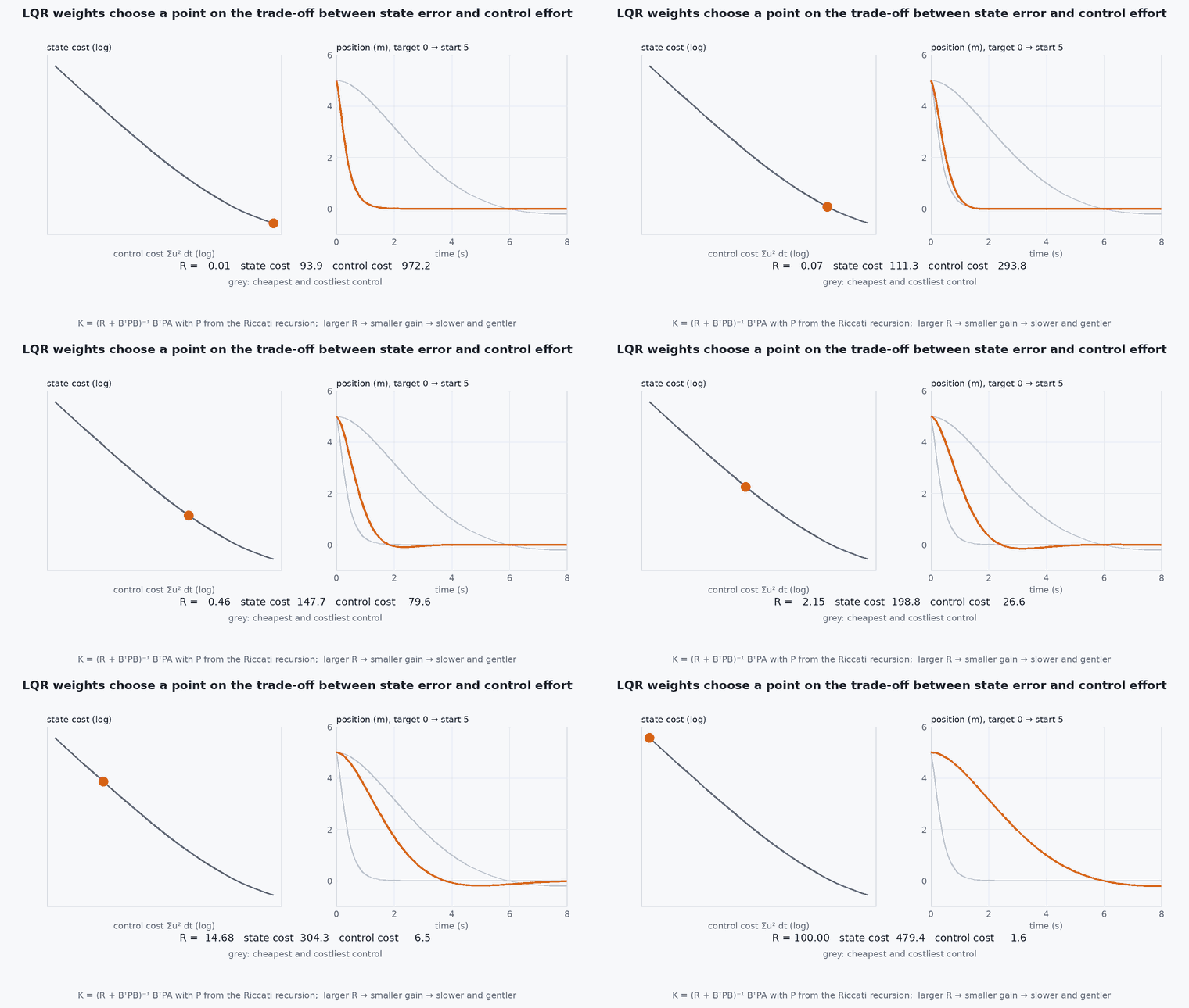
The linear-quadratic regulator minimises an infinite-horizon cost that adds up squared state error and squared control effort. For a linear model the solution is a constant state-feedback gain : . The tuning knobs are two weight matrices: says how much each state error matters, says how expensive each input is.
Unlike separate PID loops, LQR uses all states at once: it knows, for instance, that position error should be corrected through a coordinated change of velocity and tilt rather than by each loop independently.
Engineering intuition
Large on a state says “keep this near zero, even at the cost of effort”; large says “be gentle with the actuator”. The ratio sets the speed of response: heavier gives a faster, more energetic controller. Because the design is optimal for the model, it is only as good as the model: it inherits guaranteed stability margins for the ideal linear case, but real motor lag, delays and saturation reduce them, so verify in simulation with those effects before flying.
Mathematical formulation
Discrete model and cost with ⪰ 0, ≻ 0:
- state error relative to the reference (for position control: position, velocity, attitude, rate errors).
- state weights, diagonal in practice; Bryson’s rule sets /(max acceptable ).
- input weights; Bryson’s rule sets /(max acceptable ).
- cost-to-go matrix: .
Linearised hover (one horizontal axis)
About hover, with small angles and forward, , . With state and input the normalised torque :
Four integrator-chain states, one input: the pair (, ) is controllable, so an LQR exists. The solution has the cascaded look of PID (position error to velocity to tilt to rate) but with gains chosen jointly.
For reference tracking, define the error relative to the reference trajectory and add feedforward, or augment with an integrator state to reject constant disturbances (LQI).
Architecture and data flow
Design offline: linearise, discretise, choose and , solve the Riccati equation, store . Online: compute the state error from the estimator, , pass the torque (or acceleration) command to the next loop. If the estimator’s delay is significant, include it in the model, because LQR assumes the state is known exactly and instantly.
Real-world UAV applications
- Hover and position hold with coordinated multi-state feedback.
- Gain-scheduled controllers across payload or speed.
- Terminal controller and cost-to-go in MPC (the same matrix).
- Quick controller design for new airframes from CAD-derived inertia.
Implementation example
This runs as shown: it builds the discretised hover model, solves the Riccati equation by iteration (no SciPy required), and simulates the closed loop from a 2 m position error, comparing with an arbitrary hand-picked gain set.
import numpy as np
g, dt = 9.81, 0.01
Ac = np.array([[0, 1, 0, 0], [0, 0, g, 0], [0, 0, 0, 1], [0, 0, 0, 0.0]]); Bc = np.array([[0], [0], [0], [1.0]])
# zero-order-hold discretisation: A = exp(Ac dt), B = (integral of exp(Ac s) ds from 0 to dt) Bc, both by their power series
A = np.eye(4); term = np.eye(4)
for k in range(1, 6):
    term = term @ (Ac * dt) / k; A = A + term
B = np.zeros((4, 1)); Mt = np.eye(4) * dt
for k in range(6):
    B += Mt @ Bc; Mt = Mt @ (Ac * dt) / (k + 2)

def dlqr(A, B, Q, R, iters=20000):
    P = Q.copy()
    for _ in range(iters):
        K = np.linalg.solve(R + B.T @ P @ B, B.T @ P @ A)
        Pn = Q + A.T @ P @ (A - B @ K)
        if np.max(np.abs(Pn - P)) < 1e-11: P = Pn; break
        P = Pn
    return np.linalg.solve(R + B.T @ P @ B, B.T @ P @ A), P

# Bryson's rule: 1 m position, 1 m/s, 0.2 rad, 1 rad/s acceptable; input 5 rad/s^2
Q = np.diag([1 / 1.0**2, 1 / 1.0**2, 1 / 0.2**2, 1 / 1.0**2]); R = np.array([[1 / 5.0**2]])
K, P = dlqr(A, B, Q, R)
print("K =", np.round(K, 3))
rho = max(abs(np.linalg.eigvals(A - B @ K)))
assert rho < 1                                                 # closed loop is stable

def run(K, T=12.0):
    x = np.array([2.0, 0, 0, 0]); out = []
    for _ in range(int(T / dt)):
        u = np.clip(-K @ x, -30, 30)
        x = A @ x + (B @ u).ravel(); out.append(x[0])
    return np.array(out)
traj = run(K)
t_settle = np.argmax(np.abs(traj[::-1]) > 0.1 * 2.0)            # last time |x| exceeds 10% of the step
print(f"closed-loop spectral radius {rho:.4f}; position error back inside 10% after {(len(traj) - t_settle) * dt:.1f} s; final {traj[-1]:.4f} m")
assert abs(traj[-1]) < 0.01 and abs(traj.min()) < 1.0 # converges without wild undershootCommon engineering mistakes
Treating Q and R as arbitrary numbers
Use Bryson’s rule and normalise units so weights reflect acceptable errors and inputs.
Ignoring actuator limits
LQR is unconstrained; a large step saturates the motors and the guarantees disappear. Limit the setpoint or use MPC.
Using a linearisation far from its point
The hover model is valid for small angles only; schedule gains or use MPC for aggressive flight.
No integral action
A constant wind leaves a steady-state offset; use an integrator state.
Assuming perfect state knowledge
Estimator delay and noise reduce margins: simulate with them.
Failure modes
| Failure mode | How it shows up | Likely cause |
|---|---|---|
| Oscillation after saturation | Ringing after an aggressive command | Actuator limits violate the linear assumption |
| Steady-state offset in wind | Persistent position error | No integral state |
| Poor performance at high speed | Tracking degrades as tilt grows | Linearisation invalid; need scheduling or nonlinear control |
| Model mismatch instability | Real vehicle oscillates while simulation was clean | Unmodelled motor lag or delay |
Debugging approach
- Check controllability (rank of [ AB ]) and the eigenvalues of A − BK.
- Validate in simulation with the real sensor delay and motor lag before flying.
- Compare step responses with those of the PID baseline on the same plant.
- Sweep the Q/R ratio and plot response time against control effort to find a sensible compromise.
Practical exercises
- Apply Bryson’s rule for a 0.5 m position tolerance and a 0.1 rad tilt limit; compare with the example.
- Add an integral of position error as a fifth state (LQI) and test against constant wind.
- Show that scaling and by the same factor does not change .
- Compare closed-loop poles of the LQR with those of a PD cascade you tuned in lesson M5-T6.
Interview questions
Write an answer in your own words, then reveal the model answer. Nothing is sent anywhere.
Question 1
What does LQR optimise, and what do and mean?
Model answer
It minimises the sum of squared state errors weighted by plus squared control effort weighted by . Larger relative to gives a faster, more energetic response.
Question 2
What are LQR’s main limitations for UAVs?
Model answer
It assumes a linear model and no constraints. Aggressive flight, saturation, delays and model error reduce performance and margins; MPC handles constraints explicitly.
Question 3
How does LQR differ from cascaded PID?
Model answer
LQR designs all state-feedback gains jointly and optimally from a model, giving coordinated corrections; cascaded PID tunes loops independently, which is simpler and robust but not optimal.
References and further reading
Primary papers, official documentation and standards. Each claim above that is specific to a tool or version points here.
- . . . Anderson, . . Moore, Optimal Control: Linear Quadratic Methods, Prentice-Hall, 1990.
- . . Åström, . . Murray, Feedback Systems, Princeton University Press, 2008, chapter 6.
- R. Mahony, V. Kumar, P. Corke, IEEE RAM 2012