UAV Systems Engineering · Module 5
M5-T8: Model Predictive Control
MPC plans several steps ahead under constraints, applies the first move and replans: the one controller that knows its own limits.
PID reacts to the present error and LQR is optimal without constraints. MPC looks ahead along the reference and respects limits on acceleration, velocity and tilt as part of the problem. It costs computation, and the price is worth knowing before using it on a flight computer.
Learning objectives
After this lesson, you should be able to:
- Formulate a finite-horizon MPC problem and the receding-horizon principle.
- Build the condensed QP for a double-integrator UAV with input and state constraints.
- Explain the effect of prediction horizon, control horizon and weights.
- Describe model mismatch, feasibility and real-time issues.
Conceptual explanation
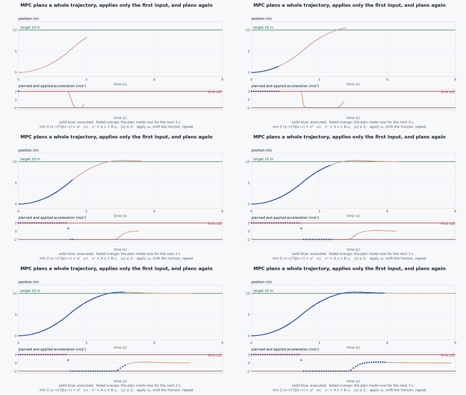
At every control step MPC solves an optimisation: choose a sequence of future inputs that minimises tracking error and effort over a horizon, subject to the model and to constraints. It applies only the first input, measures the new state, and solves again: receding horizon control.
Because the optimiser sees the reference ahead of time, it brakes before a corner; because the constraints are in the problem, it never asks for more acceleration than exists. The MPC Flight Controller Simulator shows both effects against a saturating PD baseline.
Engineering intuition
Think of a driver who looks down the road: slow before the bend because the car cannot corner faster than its grip allows. The prediction horizon is how far ahead the driver looks; if it is shorter than the braking distance, the driver cannot anticipate. The control horizon is how many separate decisions the driver plans: fewer decisions mean a cheaper but less flexible plan.
The model inside MPC is only an approximation: it ignores motor lag, wind and delays. Feedback (re-solving every step from the measured state) corrects for this, but a poor model with a long horizon plans confidently for a vehicle that does not exist. Keep the horizon long enough to anticipate and short enough that the model error over it stays small.
Mathematical formulation
Double-integrator per axis, state , input = acceleration, step :
Stack the predictions over steps with the first inputs free (the last one held): , where is lower-triangular in . The cost is:
With constraints and , the problem is a convex QP: min ½HU + subject to , where velocity constraints become linear in through :
- ,
- prediction and control horizons (steps), .
- ,
- tracking weights; , effort and move-rate weights.
- maps free inputs to predicted states.
- ,
- stacked inequality constraints.
The QP is solved by an active-set, interior-point or first-order method; the simulator uses Hildreth’s dual coordinate ascent, which is simple and exact for small problems. Production MPC for UAVs uses dedicated solvers such as OSQP, qpOASES, acados or FORCES Pro. Feasibility is a design concern: if the vehicle is already above the velocity limit, the constraints can be infeasible, so relax them (soft constraints or a feasibility margin as in the simulator).
Architecture and data flow
Estimator state → reference preview (positions and velocities over the horizon from the trajectory generator) → MPC solve (budget: a fraction of the control period) → acceleration or attitude/thrust setpoint → inner attitude loop on the flight controller. Computation time and its jitter belong in the latency budget (lesson M7-T6): an MPC that sometimes overruns its period is a real-time failure. Provide a fallback (the previous solution shifted, or a PD law) for overruns.
Real-world UAV applications
- Tracking aggressive or time-optimal trajectories within actuator limits.
- Collision-avoidance constraints in the same optimisation.
- Quadrotor racing and agile flight research (nonlinear MPC on the full dynamics).
- Payload and wind-aware tracking with disturbance estimation.
Implementation example
This runs as shown: a condensed MPC for one axis with acceleration and velocity constraints, solved with Hildreth’s method, driving the vehicle to a position step while respecting both limits.
import numpy as np
T = 0.1; A = np.array([[1, T], [0, 1]]); Bv = np.array([T**2 / 2, T])
def build(N, Nc):
    Pp = np.zeros((N, Nc)); Pv = np.zeros((N, Nc))
    for k in range(1, N + 1):
        for j in range(k):
            c = min(j, Nc - 1)
            Pp[k - 1, c] += T**2 * (k - j - 0.5); Pv[k - 1, c] += T
    return Pp, Pv

def hildreth(H, f, G, g, iters=5000):
    Hi = np.linalg.inv(H); P = G @ Hi @ G.T; d = G @ Hi @ f + g
    lam = np.zeros(len(g))
    for _ in range(iters):
        old = lam.copy()
        for i in range(len(g)):
            w = d[i] + P[i] @ lam - P[i, i] * lam[i]
            lam[i] = max(0.0, -w / P[i, i])
        if np.max(np.abs(lam - old)) < 1e-9: break
    return -Hi @ (f + G.T @ lam)

def mpc(x0, ref_p, N=20, Nc=8, qp=10.0, qv=1.0, ru=0.05, vmax=2.0, amax=1.5):
    Pp, Pv = build(N, Nc)
    free_p = np.array([x0[0] + k * T * x0[1] for k in range(1, N + 1)]); free_v = np.full(N, x0[1])
    H = qp * Pp.T @ Pp + qv * Pv.T @ Pv + ru * np.eye(Nc) + 1e-9 * np.eye(Nc)
    f = qp * Pp.T @ (free_p - ref_p) + qv * Pv.T @ free_v
    G = np.vstack([np.eye(Nc), -np.eye(Nc), Pv, -Pv])
    g = np.concatenate([np.full(Nc, amax), np.full(Nc, amax), np.full(N, vmax) - free_v, np.full(N, vmax) + free_v])
    u0 = hildreth(H, f, G, g)[0]
    return float(np.clip(u0, -amax, amax))       # dual coordinate ascent converges slowly: clip the applied move to the (box) input limit

x = np.array([0.0, 0.0]); speeds, accs = [], []
for _ in range(150):                                         # 15 s to a 10 m step
    u = mpc(x, ref_p=np.full(20, 10.0))
    x = A @ x + Bv * u; speeds.append(abs(x[1])); accs.append(abs(u))
print(f"final position {x[0]:.2f} m, peak speed {max(speeds):.2f} m/s (limit 2.0), peak accel {max(accs):.2f} m/s^2 (limit 1.5)")
assert max(speeds) <= 2.0 + 1e-3 and max(accs) <= 1.5 + 1e-9 and abs(x[0] - 10.0) < 0.2Common engineering mistakes
Horizon shorter than the braking time
The controller cannot anticipate corners or stops; extend the horizon or reduce speed.
Hard state constraints with no feasibility margin
The QP becomes infeasible after a disturbance. Use soft constraints or a relaxation scheme.
Ignoring solve-time jitter
An occasional overrun delays the command; budget worst-case solve time and provide a fallback.
Using a model that ignores dominant actuator lag
The plan assumes instantaneous acceleration; add the lag to the model or the horizon will mislead.
Tuning weights without units
Normalise by acceptable error and effort as in Bryson’s rule.
Failure modes
| Failure mode | How it shows up | Likely cause |
|---|---|---|
| Infeasible QP | Solver returns no solution or a saturated command | Initial state outside constraints or conflicting limits |
| Oscillation with long horizon | Chatter around the reference | Model mismatch or delay not modelled |
| Overrun | Occasional missed deadlines, jerky commands | Horizon or problem size too large for the compute budget |
| Constraint violation in flight | Speed above limit in wind | Constraints on the model, not the real plant, and no margin |
Debugging approach
- Log solver status, iterations and solve time per step.
- Replay the logged state into the MPC offline and check whether the constraints are active when the real vehicle misbehaves.
- Compare predicted and actual state one step later to measure model error.
- Sweep horizon length and plot tracking error against solve time.
Practical exercises
- Show that for no constraints and , MPC reduces to a linear time-invariant state feedback.
- Add a position constraint (a wall at 8 m) to the example and watch the plan stop short.
- Measure the solve time against horizon in the code and extrapolate the maximum for a 20 ms budget.
- Use the MPC Simulator’s lag slider to find where the unmodelled lag degrades tracking.
Interview questions
Write an answer in your own words, then reveal the model answer. Nothing is sent anywhere.
Question 1
What is the receding-horizon principle?
Model answer
Solve a finite-horizon optimal control problem, apply only the first control, then re-solve from the new measured state at the next step, so feedback corrects model error and disturbances.
Question 2
What do prediction and control horizons do?
Model answer
The prediction horizon is how far ahead outcomes are evaluated, which sets how early the controller anticipates; the control horizon is how many free input moves are optimised, trading flexibility for computation.
Question 3
Why is MPC computationally harder than LQR and how is that managed?
Model answer
It solves a QP at every step instead of one matrix multiply; manage with short horizons, move blocking, warm starts, fast solvers, and fallbacks for overruns.
References and further reading
Primary papers, official documentation and standards. Each claim above that is specific to a tool or version points here.
- D. Q. Mayne, J. B. Rawlings, C. V. Rao, P. O. M. Scokaert, “Constrained model predictive control: stability and optimality”, Automatica, 2000
- . . Rawlings, . . Mayne, . . Diehl, Model Predictive Control: Theory, Computation, and Design, 2nd ed., Nob Hill, 2017.
- OSQP: quadratic programming solver (documentation)