UAV Systems Engineering · Module 5
M5-T9: Trajectory generation
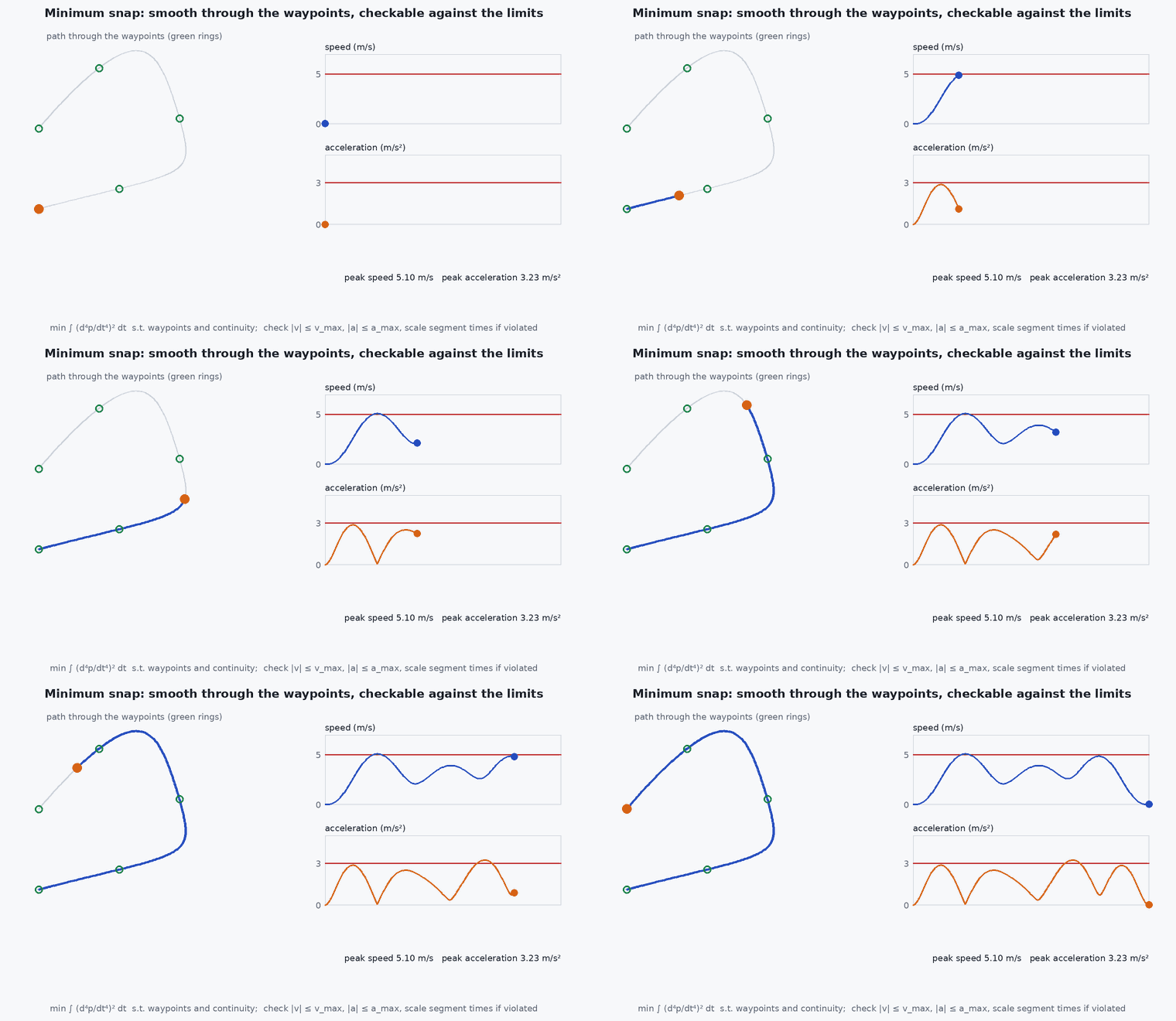
A quadrotor can follow any smooth enough path, and the smoothest one minimises snap: the fourth derivative of position.
A planner outputs waypoints; a controller needs a trajectory it can actually fly. This lesson turns the first into the second with the standard minimum-snap formulation, and shows what to check before sending it to a vehicle.
Learning objectives
After this lesson, you should be able to:
- Explain why snap is the right smoothness measure for a quadrotor (differential flatness).
- Formulate the minimum-snap problem for piecewise polynomials with waypoint and continuity constraints.
- Solve it as an equality-constrained quadratic program and verify continuity.
- Check a trajectory for actuator feasibility and choose segment times.
Conceptual explanation
A quadrotor is differentially flat in the flat outputs (, , , yaw): given a trajectory for these and their derivatives, the required attitude, thrust and body rates can be computed algebraically. Acceleration sets thrust and tilt; jerk sets body rates; snap sets the angular accelerations and so the motor-thrust changes. Minimising the integral of the squared snap therefore minimises, in a sense, the control effort needed to follow the path (Mellinger and Kumar, 2011).
Engineering intuition
Straight lines between waypoints are the shortest path but impose infinite acceleration at corners; the vehicle either slows to a stop at each corner or cuts it. A minimum-snap trajectory trades a slightly longer path for smooth motion, and tells you the speed you can carry through each waypoint. The remaining design choice is time: the polynomial will happily fly through the waypoints in 0.1 s with absurd accelerations, so segment times must be chosen (and checked) against the vehicle’s limits.
Mathematical formulation
Each segment is a polynomial of order 7: ᵏ on . The cost is the integral of squared snap:
Constraints are linear equalities : waypoint positions at the start and end of each segment; zero velocity and acceleration at the trajectory ends; and continuity of velocity, acceleration and jerk across segment joints (orders 1–3). Intermediate derivatives at waypoints are left free: that freedom is what the optimisation uses. The problem is an equality-constrained QP with the KKT system:
It is small, dense and solved directly. For dimensions, solve each independently (, , ). Time allocation: a common start is the segment length divided by a nominal speed, with a trapezoidal profile for short segments, followed by a feasibility check and rescaling.
Feasibility
Evaluate on a time grid: speed ≤ ; acceleration magnitude ≤ the horizontal acceleration the vehicle can produce (about plus margin) and thrust within limits ; jerk and snap against actuator rate limits. If violated, scale all segment times by a factor : velocity scales as 1/s, acceleration as , jerk as .
Architecture and data flow
Waypoints (from a planner or mission) → time allocation → minimum-snap solve per axis → sample at the controller rate (position, velocity, acceleration, jerk, yaw) → trajectory tracker (MPC or PID with feedforward). With PX4 offboard control, send position, velocity and acceleration setpoints in NED from the sampled trajectory at a steady rate (lesson M6-T11). Replanning must start from the vehicle’s current planned state, not its measured one, to avoid jerks.
Real-world UAV applications
- Smooth waypoint flight through cluttered environments.
- Aggressive flight and racing trajectory generation.
- Corridor-constrained trajectories after a path planner (lesson M5-T11).
- Camera-friendly motion with bounded jerk for inspection.
Implementation example
This runs as shown: a one-axis minimum-snap solve through four waypoints, verifying that the trajectory hits the waypoints and is continuous in velocity, acceleration and jerk, and that time scaling reduces acceleration as .
import numpy as np
N = 8                                                          # 7th-order polynomials: coefficients c0..c7

def coef(i, d):
    c = 1.0
    for j in range(d): c *= (i - j)
    return c
def basis(t, d): return np.array([coef(k, d) * t ** (k - d) if k >= d else 0.0 for k in range(N)])
def snap_H(T):
    H = np.zeros((N, N))
    for i in range(4, N):
        for j in range(4, N): H[i, j] = coef(i, 4) * coef(j, 4) * T ** (i + j - 7) / (i + j - 7)
    return H

def minsnap(wp, T):
    n = len(wp) - 1; H = np.zeros((N * n, N * n)); rows = []; rhs = []
    for s in range(n): H[s*N:(s+1)*N, s*N:(s+1)*N] = snap_H(T[s])
    def row(seg, t, d, other=None):
        v = np.zeros(N * n); v[seg*N:(seg+1)*N] = basis(t, d)
        if other is not None: v[other*N:(other+1)*N] -= basis(0, d)       # continuity: end of seg == start of other
        return v
    for s in range(n): rows += [row(s, 0, 0), row(s, T[s], 0)]; rhs += [wp[s], wp[s+1]]   # waypoint positions
    for d in (1, 2): rows += [row(0, 0, d), row(n-1, T[-1], d)]; rhs += [0, 0]             # rest at both ends
    for s in range(n - 1):
        for d in (1, 2, 3): rows.append(row(s, T[s], d, s + 1)); rhs.append(0)             # C3 continuity at joints
    A = np.array(rows); b = np.array(rhs); m = len(b)
    K = np.block([[2 * H + 1e-9 * np.eye(N * n), A.T], [A, np.zeros((m, m))]])
    return np.linalg.solve(K, np.concatenate([np.zeros(N * n), b]))[:N * n].reshape(n, N)

wp, T = [0.0, 2.0, 1.0, 3.0], [1.5, 1.5, 1.5]
C = minsnap(wp, T)
for s in range(3):
    assert abs(basis(0, 0) @ C[s] - wp[s]) < 1e-8 and abs(basis(T[s], 0) @ C[s] - wp[s + 1]) < 1e-8      # passes through every waypoint
for s in range(2):
    for d in (1, 2, 3): assert abs(basis(T[s], d) @ C[s] - basis(0, d) @ C[s + 1]) < 1e-6             # continuity
def peak_acc(C, T, scale=1.0):
    return max(abs(basis(t, 2) @ C[s]) for s in range(len(T)) for t in np.linspace(0, T[s], 200)) / scale ** 2
C2 = minsnap(wp, [2 * t for t in T])                                                                     # stretch every segment time by s = 2
a1, a2 = peak_acc(C, T), peak_acc(C2, [2 * t for t in T])
print(f"peak acceleration {a1:.2f} m/s^2; with all times doubled {a2:.2f} (ratio {a1 / a2:.2f}, expected 4)")
assert abs(a1 / a2 - 4) < 0.05Common engineering mistakes
Ignoring segment times
The polynomial is feasible mathematically and impossible physically. Always evaluate speed, acceleration and thrust along it.
Solving in the wrong frame or forgetting gravity
Thrust is , not .
Numerically unstable high-order monomials over long segments
Use normalised time per segment (0 to 1) or a Bernstein basis for many segments.
Replanning from the measured state
Introduces jerk; start from the previous planned state.
Treating waypoints as hard when clearances are soft
A smooth curve cuts corners: constrain it to a collision-free corridor (lesson M5-T11).
Failure modes
| Failure mode | How it shows up | Likely cause |
|---|---|---|
| Corner cutting | Trajectory passes through obstacles between waypoints | No corridor constraint; smoothness overrides geometry |
| Aggressive overshoot | Large excursions between two close waypoints | Unbalanced segment times |
| Infeasible acceleration | Tracker saturates, large tracking error | Times too short for the geometry |
| Ill-conditioned solve | NaN or wild coefficients | High-order polynomial over long durations without normalisation |
Debugging approach
- Plot position, velocity, acceleration and jerk against their limits for each axis and in 3-D magnitude.
- Check each waypoint is hit to 1e-8 and joints are continuous.
- Scale all times by a factor and check the law.
- Simulate the tracker on the trajectory before flying it.
Practical exercises
- Allocate segment times from distances and a 2 m/s cruise speed, then find the scale needed to keep acceleration below .
- Extend the solver to 3-D and plot the path.
- Add a velocity constraint at a waypoint and see how the cost changes.
- Compare snap cost against the piecewise-cubic spline through the same waypoints.
Interview questions
Write an answer in your own words, then reveal the model answer. Nothing is sent anywhere.
Question 1
Why minimise snap rather than acceleration or jerk?
Model answer
Because a quadrotor is differentially flat: acceleration gives thrust and tilt, jerk gives body rates, and snap gives angular accelerations and so the changes in motor thrust, so minimising snap minimises the control effort needed.
Question 2
How do you make a minimum-snap trajectory feasible?
Model answer
Choose segment times, evaluate speed, acceleration and thrust along the result, and stretch times (acceleration scales as ) until limits hold, adding corridor constraints for obstacles.
Question 3
What are the constraints in the QP?
Model answer
Waypoint positions, boundary derivatives at the ends, and continuity of derivatives up to jerk across joints; intermediate derivatives are free for the optimiser.
References and further reading
Primary papers, official documentation and standards. Each claim above that is specific to a tool or version points here.