UAV Systems Engineering · Module 3
M3-T15: Normalized Estimation Error Squared
NIS needs no ground truth and tests the measurements; NEES needs ground truth and tests the state estimate itself. Together they tell you whether a filter is honest.
A filter that is accurate but overconfident is dangerous: a planner or monitor trusting its covariance will take risks the data do not support. NEES is the test for that, and simulation is where you can run it.
Learning objectives
After this lesson, you should be able to:
- Define NEES and the distribution it follows for a consistent filter.
- Run a Monte Carlo consistency test and compute average NEES with chi-square bounds.
- Interpret values above and below the band and relate them to , and model error.
- Explain why NEES is a simulation tool and what replaces it in flight.
Conceptual explanation
The normalised estimation error squared compares the actual error of the state estimate with the covariance the filter reports: NEES = . If the filter is consistent, the error is zero-mean Gaussian with covariance and NEES is chi-square with degrees of freedom (the state dimension), so its mean is .
It needs the true state, so it is a simulation and test-range tool. Onboard, where truth is unavailable, NIS (lesson M3-T14) and cross-checks between sensors take its place.
Engineering intuition
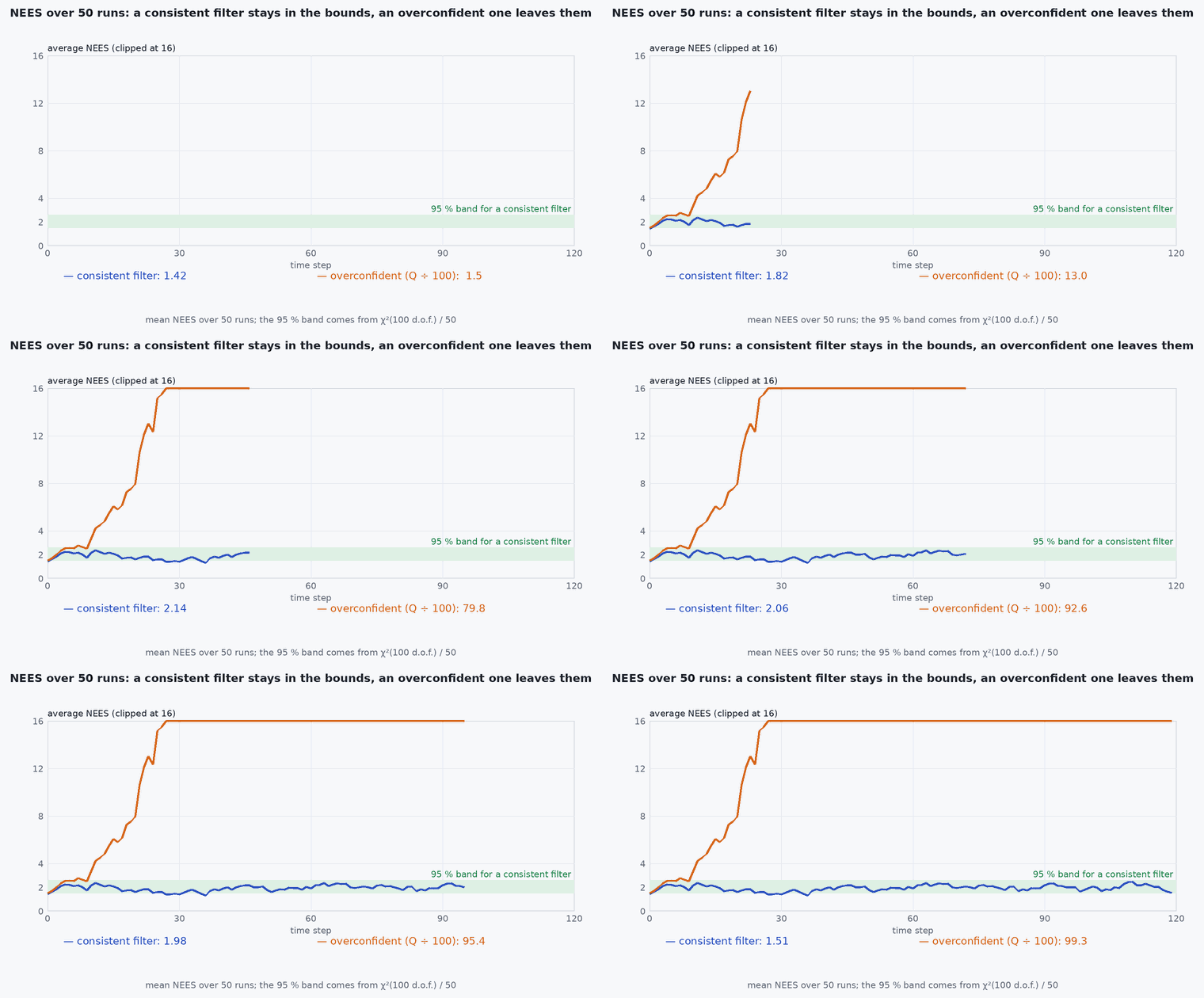
The covariance is a promise: “my error is probably within this ellipse”. NEES counts how often and by how much the promise is broken. A mean far above means the errors are larger than promised (overconfident): the covariance is too small, which usually means or too small, an unmodelled error, or a linearisation problem. A mean far below means the filter is needlessly pessimistic. One run proves little because a single trajectory is a sample of one; averaging independent runs reduces the variance of the test by .
Mathematical formulation
For independent runs, the average NEES at time has degrees of freedom after scaling:
- dimension of the state (or of the sub-state tested, for example position only).
- number of independent Monte Carlo runs with different noise seeds.
- significance level, typically 0.05 for a 95% two-sided band.
For large degrees of freedom the chi-square quantile is well approximated by the Wilson–Hilferty formula , with the standard normal quantile (±1.96 for 95%). Test position and velocity sub-blocks separately as well: a consistent total NEES can hide an inconsistent sub-block.
Architecture and data flow
Simulation harness: generate truth → simulate sensors with exactly the noise the filter assumes → run the filter times with different seeds → record error and covariance per step → compute the average NEES and its bounds → plot. First do this with perfectly matched models (it must pass: otherwise the filter or the test is wrong), then with realistic mismatch (the interesting result is how far outside the band it goes).
Real-world UAV applications
- Validating a new estimator before flight.
- Tuning and against truth in simulation, then confirming with NIS on logs.
- Regression tests that fail when a code change makes a filter overconfident.
- Justifying that a reported covariance can be used for safety margins (lesson M2-T16).
Implementation example
This runs as shown: 100 Monte Carlo runs of a constant-velocity Kalman filter, with a matched model (passes) and a filter whose process noise is 100 times too small (fails).
import numpy as np
dt, n, runs = 0.1, 200, 100
F = np.array([[1, dt], [0, 1]]); H = np.array([[1.0, 0.0]])
q_true, r_std = 0.5, 2.0
Q = lambda q: q * np.array([[dt**3 / 3, dt**2 / 2], [dt**2 / 2, dt]]); R = np.array([[r_std**2]])

def mc_nees(q_filter, seed0=0):
    acc = np.zeros(n)
    for i in range(runs):
        rng = np.random.default_rng(seed0 + i); L = np.linalg.cholesky(Q(q_true))
        x = np.array([0.0, 5.0]); xh = x.copy(); P = np.diag([4.0, 4.0])      # filter starts with truthful uncertainty
        for k in range(n):
            x = F @ x + L @ rng.standard_normal(2)
            z = x[0] + r_std * rng.standard_normal()
            xh = F @ xh; P = F @ P @ F.T + Q(q_filter)
            S = H @ P @ H.T + R; K = P @ H.T @ np.linalg.inv(S)
            xh = xh + (K @ (z - H @ xh)).ravel(); I_KH = np.eye(2) - K @ H; P = I_KH @ P @ I_KH.T + K @ R @ K.T
            e = x - xh; acc[k] += e @ np.linalg.inv(P) @ e
    return acc / runs

def chi2_bounds(dof, z=1.96):                                           # Wilson-Hilferty approximation of the 95% interval
    f = lambda zz: dof * (1 - 2 / (9 * dof) + zz * np.sqrt(2 / (9 * dof))) ** 3
    return f(-z), f(z)

lo, hi = (b / runs for b in chi2_bounds(runs * 2))
good, bad = mc_nees(q_true)[50:], mc_nees(0.01 * q_true)[50:]
print(f"band [{lo:.2f}, {hi:.2f}] (expected 2); matched: mean {good.mean():.2f}, {100 * np.mean((good >= lo) & (good <= hi)):.0f}% in band; "
      f"Q 100x too small: mean {bad.mean():.2f}, {100 * np.mean((bad >= lo) & (bad <= hi)):.0f}% in band")
assert np.mean((good >= lo) & (good <= hi)) > 0.8 and good.mean() < 2.2
assert bad.mean() > 3 * good.mean() and np.mean(bad > hi) > 0.9Common engineering mistakes
Running one trajectory
A single run has a huge variance; use at least 20–50 runs with different seeds.
Testing with noise the filter does not assume
Unmatched noise tests a different question. First pass the matched case.
Looking only at total NEES
Test position and velocity (and attitude) blocks separately.
Using NEES onboard
Truth is not available in flight; use NIS and cross-checks there.
Tuning only to get NEES inside the band
Inflating blindly passes the test and wastes information; tune and from physics and logs.
Failure modes
| Failure mode | How it shows up | Likely cause |
|---|---|---|
| Overconfident filter | Average NEES far above | or too small, linearisation error, unmodelled bias |
| Conservative filter | Average NEES below the band | or too large or double-counted noise |
| Inconsistent attitude block | Position fine, orientation NEES high | Unobservable yaw drift not reflected in |
| Initial transient outside band | High NEES in the first seconds | Initial covariance too small for the initial error |
Debugging approach
- Plot average NEES versus time for each block with the band.
- Check the matched case first; if it fails, suspect the Jacobian, the discretisation of or a covariance-update bug.
- Plot error against ± for the worst block.
- Repeat with the sensor and process noise you believe real and see how far the result moves.
Practical exercises
- Compute the 95% band for and runs.
- Run the example with mis-scaled by 4 in both directions and report NEES.
- Test position alone in the example: is its average NEES consistent?
- Apply the harness to the Sensor Fusion simulator’s VIO covariance.
Interview questions
Write an answer in your own words, then reveal the model answer. Nothing is sent anywhere.
Question 1
What does NEES test that NIS does not?
Model answer
NEES compares the actual state error with the reported covariance, testing the estimate itself; NIS only tests the measurement residuals and needs no truth. A filter can pass NIS and still be inconsistent in unobservable states.
Question 2
Why average over Monte Carlo runs?
Model answer
One run is a single sample; averaging runs reduces the test variance so the chi-square band is tight enough to detect inconsistency.
Question 3
What does an average NEES well above mean in practice?
Model answer
The filter is overconfident: real errors exceed its reported uncertainty, so anything using that covariance (gates, planners, monitors) will be too trusting.
References and further reading
Primary papers, official documentation and standards. Each claim above that is specific to a tool or version points here.
- . Bar-Shalom, . . Li, . Kirubarajan, Estimation with Applications to Tracking and Navigation, Wiley, 2001, section 5.4 (consistency tests).
- . . Barfoot, State Estimation for Robotics, Cambridge University Press, 2017.
- OpenVINS documentation: evaluation and consistency (NEES) tooling