UAV Systems Engineering · Module 4
M4-T12: Pose graph optimization
Odometry drifts, loop closures pull it back: pose graph optimisation is the least-squares problem that reconciles them.
SLAM back-ends such as those in ORB-SLAM3 and VINS-Fusion correct drift by solving a graph of relative-pose constraints. The idea is small enough to implement in a page of code, and seeing it work explains both its power and its main failure mode, the false loop closure.
Learning objectives
After this lesson, you should be able to:
- Define the pose graph, its edges and information matrices.
- Write the least-squares objective and one Gauss–Newton step.
- Explain the sparsity that makes large graphs tractable and the role of robust kernels.
- Run a loop-closure optimisation and measure the drift removed.
Conceptual explanation
A pose graph has one node per estimated pose and one edge per measurement of a relative pose between two nodes: odometry edges between consecutive poses and loop-closure edges between poses that observed the same place. Odometry alone gives a chain whose errors accumulate; a loop closure supplies a constraint that does not depend on the path in between, and optimisation spreads the correction along the loop.
Engineering intuition
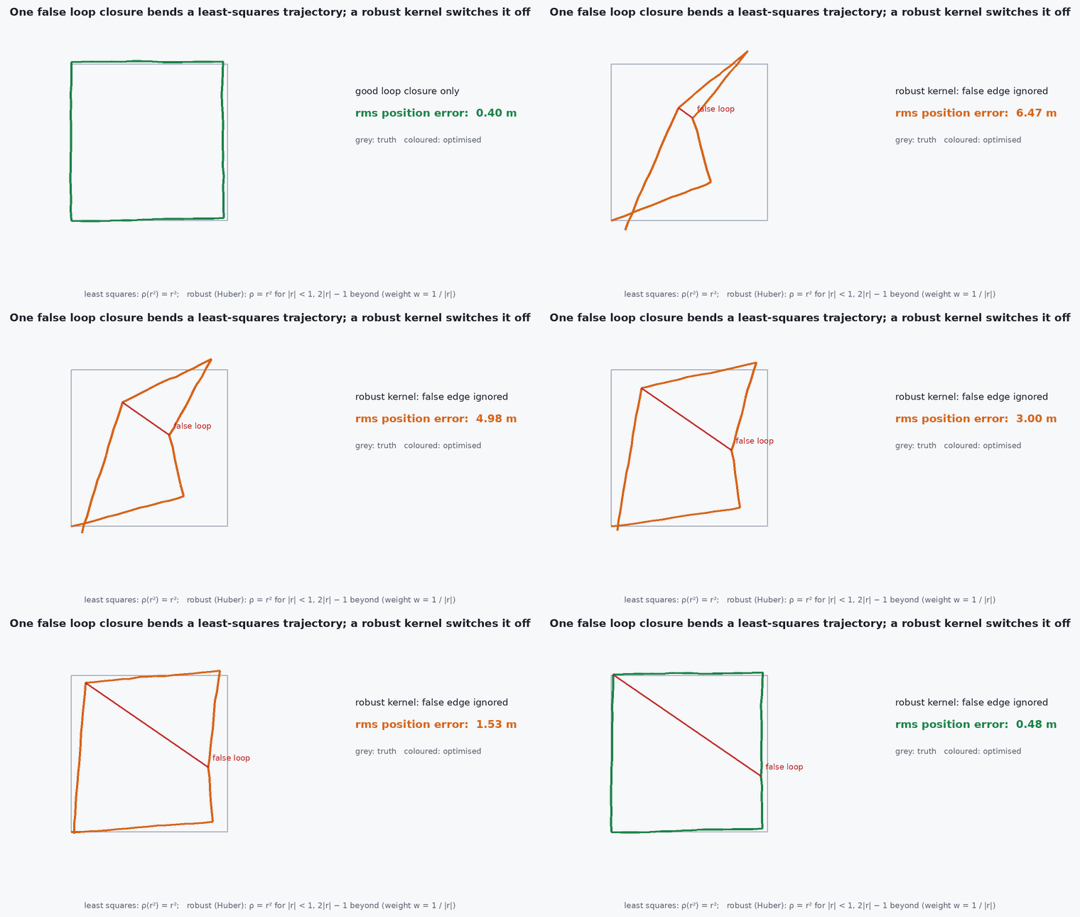
Picture a chain of springs, each with a rest length given by its measurement and a stiffness given by its information. Hold the first pose fixed and add the loop-closure spring between the last and the first: the chain stretches slightly everywhere to satisfy all springs at minimum total energy. Stiff (precise) edges move little; soft edges absorb the correction. A wrong loop closure is a spring attached to the wrong place: it distorts the whole map, which is why loop candidates are verified geometrically and why robust kernels are used.
Mathematical formulation
For poses and a measured relative pose with information matrix (inverse covariance), the residual is the difference between the measurement and the predicted relative pose, and the problem is:
In SE(2), with relative pose written in the frame of : = [ᵢ, ]. Gauss–Newton linearises and solves:
Each edge involves only two nodes, so is sparse and is a sparse block matrix whose structure is the graph: large graphs (tens of thousands of poses) are solved with sparse Cholesky (g2o, GTSAM, Ceres). The solution is defined up to a global rigid transform, so one pose is fixed (a gauge constraint, the anchor).
Robust kernels
Replace the squared error by a robust function (Huber, Cauchy, switchable constraints) so that one bad loop closure cannot dominate. Robustness reduces damage but does not replace geometric verification of loop candidates.
Architecture and data flow
Front-end: odometry (VIO or LIO) gives relative-pose edges; place recognition proposes loop candidates; geometric verification (registration or PnP with RANSAC) accepts or rejects them and produces relative-pose edges with covariance. Back-end: the optimiser updates all poses; the map (keyframes, points) is re-anchored. For a UAV in flight, a global correction changes the pose estimate abruptly: feed it to the controller through a smoothing layer, keep the local odometry frame continuous, and publish the correction as a transform between a map frame and an odom frame (as in the ROS convention).
Real-world UAV applications
- Loop closure in ORB-SLAM3 and VINS-Fusion back-ends.
- Merging maps from multiple flights or multiple vehicles.
- Fusing GNSS as absolute-position edges when available.
- Offline refinement of a mapping flight before using the map for localisation (lesson M4-T13).
Implementation example
This runs as shown: a 40-pose square loop with biased, noisy odometry. Optimising with one loop-closure edge removes most of the drift. Numerical Jacobians keep the example short; real systems use analytic ones and sparse solvers.
import numpy as np
rng = np.random.default_rng(1)
wrap = lambda a: (a + np.pi) % (2 * np.pi) - np.pi
def rel(a, b):                                   # pose b expressed in the frame of pose a
    d = b[:2] - a[:2]; c, s = np.cos(a[2]), np.sin(a[2])
    return np.array([c * d[0] + s * d[1], -s * d[0] + c * d[1], wrap(b[2] - a[2])])
def comp(a, u):                                  # pose a composed with the relative motion u
    c, s = np.cos(a[2]), np.sin(a[2])
    return np.array([a[0] + c * u[0] - s * u[1], a[1] + s * u[0] + c * u[1], wrap(a[2] + u[2])])

n = 40; truth = [np.zeros(3)]                    # square loop: 1 m steps, a 90-degree turn every 10 steps
for k in range(n): truth.append(comp(truth[-1], np.array([1.0, 0, np.pi / 2 if (k + 1) % 10 == 0 else 0.0])))
truth = np.array(truth)
odo = [rel(truth[k], truth[k + 1]) + np.array([0.02, 0.01, 0.01]) * rng.standard_normal(3) + np.array([0, 0, 0.004]) for k in range(n)]   # noise plus a heading bias
x = [np.zeros(3)]
for u in odo: x.append(comp(x[-1], u))
x = np.array(x)
w = np.array([1 / 0.02, 1 / 0.02, 1 / 0.01])
edges = [(k, k + 1, odo[k], w) for k in range(n)] + [(n, 0, rel(truth[n], truth[0]), 5 * w)]    # last edge: loop closure from place recognition

def residual(xf):
    X = xf.reshape(-1, 3); r = []
    for i, j, z, wt in edges:
        e = rel(X[i], X[j]) - z; e[2] = wrap(e[2]); r.append(e * np.sqrt(wt))
    r.append(X[0] * 1e3)                          # anchor the first pose (gauge)
    return np.concatenate(r)

xf = x.copy().ravel()
for it in range(20):                              # Gauss-Newton with numerical Jacobians
    r = residual(xf); J = np.zeros((len(r), len(xf)))
    for k in range(len(xf)):
        xp = xf.copy(); xp[k] += 1e-6; J[:, k] = (residual(xp) - r) / 1e-6
    dx = np.linalg.solve(J.T @ J + 1e-9 * np.eye(len(xf)), -J.T @ r); xf += dx
    if np.linalg.norm(dx) < 1e-8: break
X = xf.reshape(-1, 3)
err = lambda P: np.mean(np.linalg.norm(P[:, :2] - truth[:, :2], axis=1))
print(f"mean position error: odometry {err(x):.3f} m -> optimised {err(X):.3f} m; end-point error {np.linalg.norm(x[-1,:2]-truth[-1,:2]):.3f} -> {np.linalg.norm(X[-1,:2]-truth[-1,:2]):.4f} m")
assert err(X) < err(x) / 4 and np.linalg.norm(X[-1, :2] - truth[-1, :2]) < 0.01Common engineering mistakes
Accepting loop closures without geometric verification
A single false loop can fold the whole map; verify and use robust kernels.
Forgetting the anchor
The system is under-constrained (gauge freedom): the solver drifts or fails.
Wrong information weighting
Edges with inflated confidence dominate; derive weights from sensor covariance.
Wrapping angles incorrectly
Heading residuals must be wrapped to .
Applying the correction as a jump to the controller
Publish it as a map-to-odom transform and smooth it.
Failure modes
| Failure mode | How it shows up | Likely cause |
|---|---|---|
| False loop closure | Map suddenly distorted or folded | Perceptual aliasing in repeated structures, bad verification |
| No correction at the end | Drift persists after a return to the start | No loop detected: place recognition failed or viewpoint changed |
| Slow solve | Optimisation time grows with the map | Dense solver on a large graph; use sparse solvers and keyframe pruning |
| Local minimum | Optimisation gets stuck with large initial error | Poor initial guess with large heading error; use a robust initialisation |
Debugging approach
- Plot the graph before and after optimisation with edge residuals coloured.
- Check each loop edge’s residual after convergence: large values flag bad closures.
- Run with and without the loop edge and compare the end-point error.
- Test the optimiser on synthetic data with known truth, as above.
Practical exercises
- Add a second, deliberately wrong loop closure and observe the damage, then add a Huber kernel.
- Replace numerical Jacobians with analytic ones and compare run time.
- Make the heading bias 0.02 rad per step and see how the end-point error changes.
- Count the non-zero blocks of for the example and explain the sparsity pattern.
Interview questions
Write an answer in your own words, then reveal the model answer. Nothing is sent anywhere.
Question 1
What is a pose graph and why does it help?
Model answer
Nodes are poses, edges are relative-pose measurements; loop closures add constraints independent of the drifted path, and least-squares optimisation distributes the correction along the loop.
Question 2
Why is a false loop closure so harmful?
Model answer
It is a strong constraint pulling two unrelated places together, distorting every pose between them; hence geometric verification and robust kernels.
Question 3
Why is the problem sparse?
Model answer
Each edge connects only two nodes, so the Jacobian and normal matrix have a structure mirroring the graph, enabling sparse solvers for very large maps.
References and further reading
Primary papers, official documentation and standards. Each claim above that is specific to a tool or version points here.