UAV Systems Engineering · Module 4
M4-T13: Map-based localization
With a map in hand, localisation becomes a drift-free correction: but only if you can find where you are on the map in the first place.
A prior map gives a global reference that bounds drift, unlike odometry. The problems change from accumulating error to global initialisation, ambiguity and map change. This lesson implements Monte Carlo localisation and states the conditions under which it works.
Learning objectives
After this lesson, you should be able to:
- Distinguish global localisation, pose tracking and relocalisation.
- Implement a particle filter for localisation against an occupancy map and verify convergence.
- Compare MCL with scan-to-map registration (ICP, NDT) for tracking.
- Explain failure modes: symmetry, map change and the kidnapped robot problem.
Conceptual explanation
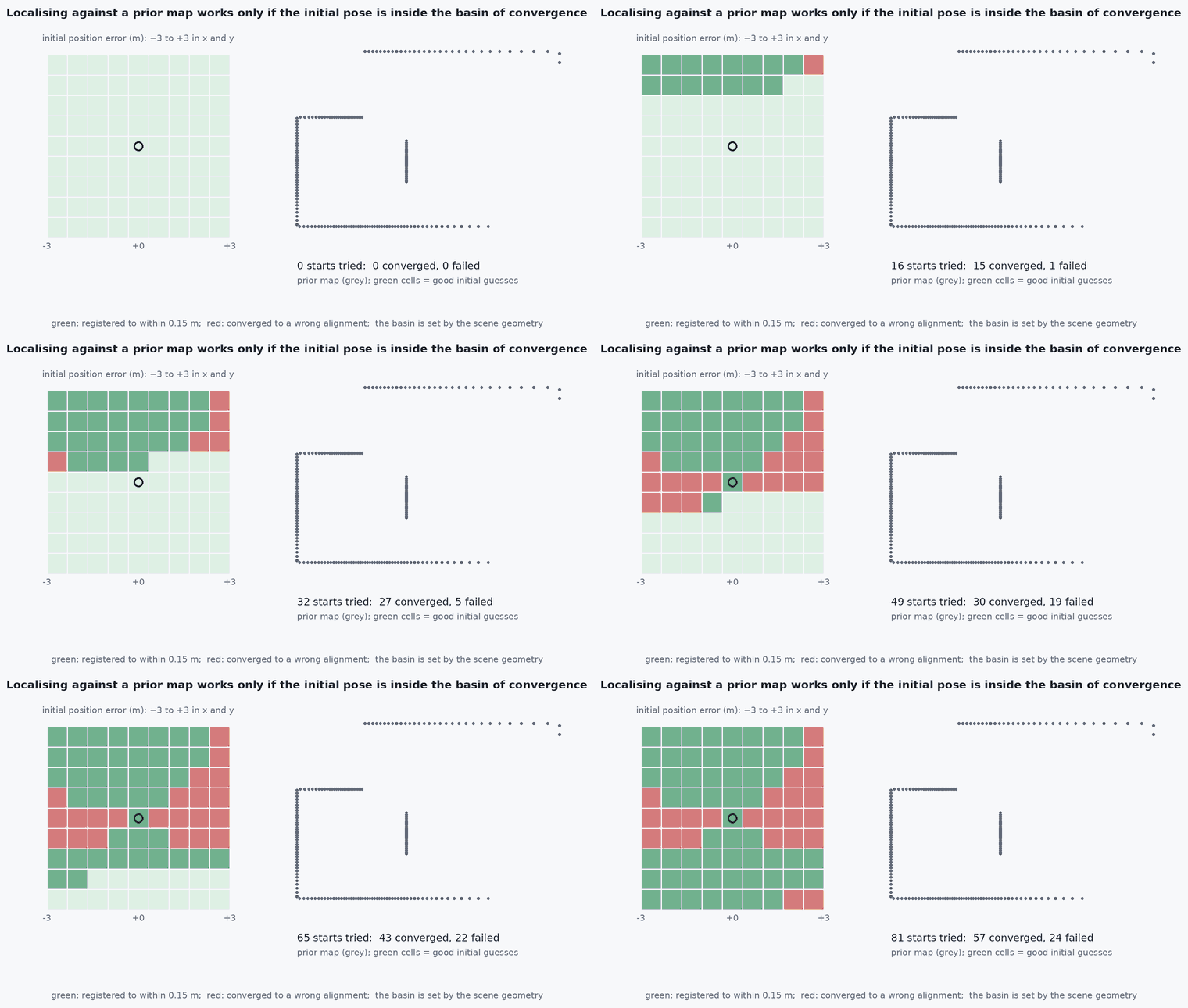
Given a map, localisation estimates the vehicle pose in the map frame. Global localisation starts with no knowledge of the pose and may face multiple hypotheses; pose tracking starts from a good guess and refines it, typically by registering sensor data to the map (ICP, NDT); relocalisation recovers after loss. Monte Carlo localisation (MCL, the particle filter, used for example in the ROS AMCL package) handles all three because it represents a multimodal belief.
Engineering intuition
Early on, many places look alike (a long corridor, symmetric rooms) and the particle cloud has several clusters. As the vehicle moves, hypotheses that predict the wrong measurements lose weight until one cluster remains. A symmetric environment may never disambiguate: then the cloud stays multimodal, and the localisation module must say so rather than report a mean between the modes. Map change (moved furniture, new obstacles) and dynamic objects reduce the likelihood of the true pose; robust measurement models and a small fraction of random particles (for recovery from kidnapping) are the standard remedies.
Mathematical formulation
For each particle with pose , the weight is the measurement likelihood given the map; in the beam model with expected ranges from ray casting and noise :
Tracking by registration minimises the distance between the scan points and the map: ICP (nearest points, lesson M2-T14) or NDT (the map as a grid of local Gaussians, maximising the likelihood of the transformed points, Biber and Straßer 2003), initialised from odometry. Number of particles: sufficient to cover the initial uncertainty (thousands for global localisation, tens to hundreds for tracking). Adaptive schemes (KLD sampling) adjust .
- expected range of beam from pose in map .
- effective number of particles, a degeneracy indicator.
Architecture and data flow
Prior map (occupancy grid, point-cloud map, voxel map) → localiser (MCL or scan-to-map) → pose in the map frame with covariance and a confidence value → published as the map-to-odom transform so the controller keeps using the smooth odom frame (lesson M4-T1). The initial pose can come from GNSS, a marker or an operator. A UAV adds the third dimension and altitude: use 3-D maps and 6-D tracking (lessons M4-T6, M4-T8).
Real-world UAV applications
- Repeatable inspection routes in a known facility.
- Drift-free indoor navigation against a surveyed map.
- Relocalisation after sensor dropout.
- Providing an absolute reference to a GNSS-denied estimator (Capstone 2).
Implementation example
This runs as shown: global localisation in a 2-D occupancy map with 16-beam range scans. Starting with particles spread uniformly, the estimate converges to within a few centimetres of the truth. Ray casting is vectorised over all particles.
import numpy as np
rng = np.random.default_rng(0)
W, H = 20, 14
grid = np.zeros((H, W), bool); grid[0, :] = grid[-1, :] = True; grid[:, 0] = grid[:, -1] = True
grid[4:8, 6] = True; grid[9, 10:15] = True; grid[3:6, 13] = True                     # an asymmetric room with obstacles
beams = np.linspace(0, 2 * np.pi, 16, endpoint=False); STEPS = np.arange(0.1, 12.0, 0.1)

def ranges(poses):                                                                    # expected ranges for many poses: (n, 16)
    ang = poses[:, 2:3] + beams[None, :]                                              # (n, 16)
    gx = np.floor(poses[:, 0, None, None] + STEPS[None, None, :] * np.cos(ang)[..., None]).astype(int)
    gy = np.floor(poses[:, 1, None, None] + STEPS[None, None, :] * np.sin(ang)[..., None]).astype(int)
    inside = (gx >= 0) & (gx < W) & (gy >= 0) & (gy < H)
    hit = ~inside | grid[np.clip(gy, 0, H - 1), np.clip(gx, 0, W - 1)]
    first = np.where(hit.any(-1), hit.argmax(-1), len(STEPS) - 1); return STEPS[first]

free = np.argwhere(~grid); N = 800
idx = rng.integers(0, len(free), N)
parts = np.stack([free[idx, 1] + rng.random(N), free[idx, 0] + rng.random(N), rng.uniform(-np.pi, np.pi, N)], axis=1)   # uniform over free space and heading
truth = np.array([3.5, 10.5, 0.5]); errs = []
for k in range(50):
    z = ranges(truth[None])[0] + 0.1 * rng.standard_normal(16)
    u = np.array([0, 0, 0.6]) if z[0] < 1.2 else np.array([0.4, 0, 0.05])             # simple wall-avoiding command, known to the filter
    truth = truth + np.array([u[0] * np.cos(truth[2]), u[0] * np.sin(truth[2]), u[2]])
    parts[:, 0] += u[0] * np.cos(parts[:, 2]) + 0.03 * rng.standard_normal(N); parts[:, 1] += u[0] * np.sin(parts[:, 2]) + 0.03 * rng.standard_normal(N); parts[:, 2] += u[2] + 0.03 * rng.standard_normal(N)
    z = ranges(truth[None])[0] + 0.1 * rng.standard_normal(16)
    gx, gy = np.floor(parts[:, 0]).astype(int), np.floor(parts[:, 1]).astype(int)
    ok = (gx >= 0) & (gx < W) & (gy >= 0) & (gy < H); ok[ok] &= ~grid[gy[ok], gx[ok]]
    ll = np.where(ok, -0.5 * (((ranges(parts) - z) / 0.3) ** 2).sum(1), -1e9)
    w = np.exp(ll - ll.max()); w /= w.sum()
    errs.append(np.linalg.norm(np.array([np.sum(w * parts[:, 0]), np.sum(w * parts[:, 1])]) - truth[:2]))
    parts = parts[rng.choice(N, N, p=w)]
print(f"position error: first update {errs[0]:.2f} m, after 10 updates {errs[9]:.2f} m, last 10 median {np.median(errs[-10:]):.3f} m")
assert errs[0] > 0.3 and np.median(errs[-10:]) < 0.1Common engineering mistakes
Reporting the mean of a multimodal cloud
It lands between the modes in free space or in a wall: report modality.
No recovery particles
After a kidnapping or map change the filter never recovers.
Too few particles for global localisation
The true hypothesis is never sampled.
Ignoring map change
Moved objects lower the true pose likelihood: use robust beam models.
Initialising with GNSS in a place with a bad fix
A wrong initial pose looks confident.
Failure modes
| Failure mode | How it shows up | Likely cause |
|---|---|---|
| Symmetric ambiguity | Pose flips between mirrored hypotheses | Symmetric environment |
| Kidnapped robot | Filter confident and wrong after relocation | No random injection |
| Map mismatch | Poor weights | Map out of date |
| Particle deprivation | Cloud collapses to a wrong pose | Too sharp likelihood or too few particles |
Debugging approach
- Plot the particle cloud over the map over time.
- Monitor and the likelihood of the best particle.
- Test with a deliberately wrong initial pose.
- Compare localisation against ground truth.
Practical exercises
- Add 5% random particles each step and test recovery after moving the truth to another room.
- Plot against time in the example.
- Replace the beam likelihood with a robust one that tolerates 20% outlier beams.
- Explain NDT in one paragraph and its advantage over ICP for tracking.
Interview questions
Write an answer in your own words, then reveal the model answer. Nothing is sent anywhere.
Question 1
What are the three localisation problems?
Model answer
Global localisation (unknown start, possibly multimodal), pose tracking (known start, refine), and relocalisation after loss (kidnapping).
Question 2
Why use particles?
Model answer
They represent multimodal beliefs and nonlinear, non-Gaussian measurement models, unlike a single Gaussian.
Question 3
How does a symmetric environment affect MCL?
Model answer
The belief stays multimodal because several poses predict the same measurements; the system must report the ambiguity and use motion or another sensor to disambiguate.
References and further reading
Primary papers, official documentation and standards. Each claim above that is specific to a tool or version points here.
- . Thrun, . Burgard, . Fox, Probabilistic Robotics, MIT Press, 2005, chapter 8.
- P. Biber, W. Straßer, “The normal distributions transform: a new approach to laser scan matching”, IROS 2003
- Nav2 AMCL (adaptive Monte Carlo localisation)