UAV Systems Engineering · Module 7
M7-T10: Software timestamping
A timestamp is a measurement with an error budget. Know where yours comes from and bound it.
Not every sensor can be hardware-triggered. For the rest, the timestamp is a software measurement taken some time after the event. The error is mostly a fixed delay (which can be calibrated) plus a variable delay (which can be reduced, but not removed). This lesson is about making that budget explicit.
Learning objectives
After this lesson, you should be able to:
- List the sources of timestamp delay between the physical event and the message header.
- Choose the stamping point (device, driver, kernel, application) appropriate to the accuracy needed.
- Reduce arrival-time jitter with a fitted period model and quantify the remaining error.
- Estimate a constant sensor-to-host delay from data and verify it.
Conceptual explanation
Established Delay sources and smoothing methods are standard in sensor integration. The size of each delay is device-specific: the example numbers are illustrative and must be replaced by measurements of your sensors.
Where each delay comes from, with who can fix it:
| Stage | Typical effect | Remedy |
|---|---|---|
| Exposure / integration | The sample represents an interval, not an instant (camera exposure; IMU filter group delay) | Stamp the midpoint; model filter delay |
| Readout and transfer | Fixed (readout) plus variable (bus arbitration) delay | Device timestamps, or calibrate the fixed part |
| Driver and kernel queue | Interrupt latency, buffering, batching of packets | Kernel or device timestamps (SO_TIMESTAMPING, hardware timestamps), real-time priority |
| Application | Scheduling delay before the callback calls now() | Stamp in the driver at the earliest point; avoid stamping in a busy callback |
Sensors differ in what they offer: some provide device timestamps on a device clock (many IMUs, lidars, some cameras), which are precise but on a different clock to be related to the host; others provide nothing and the driver stamps on arrival. A device clock can be related to the host clock by fitting: collect pairs (device time, host arrival time), whose lower envelope is the true offset plus the minimum delay.
Engineering intuition
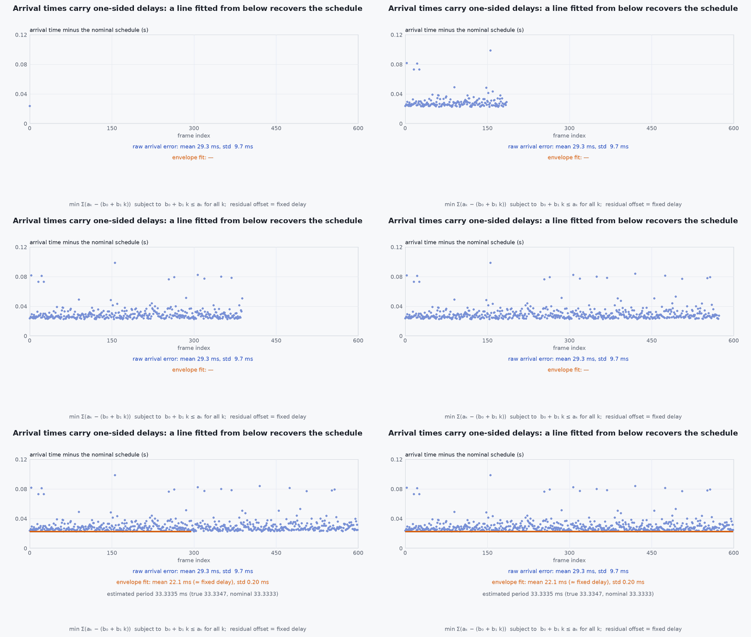
Arrival times are the true schedule plus a one-sided, positive delay with a long tail: data cannot arrive earlier than physics allows, but it can arrive late for many reasons. Because the delay is one-sided, averaging arrival times biases the answer late, and the good information is in the early arrivals. If the sensor runs at a steady rate, fit a straight line to arrival times against sample index, then pull the line down so that it sits under (almost) all the arrivals: the line is your best estimate of when the samples actually left the sensor, plus the minimum delay.
The remaining unknown is the fixed delay (readout, transfer). It is the same for every sample, so it behaves like a constant time offset that can be calibrated against another sensor (for example camera-IMU offset estimation) or measured with a hardware reference such as an LED or a sync pulse.
Mathematical formulation
For samples at nominal period indexed , with arrival times (ηk ≥ 0 variable delay, fixed delay, the sensor’s actual period, which differs from the nominal one by clock drift), the estimate of the grid is the line that minimises the sum of the residuals subject to being below all points (a linear program, solved as a lower convex hull; the “convex hull” timestamp filter), or more robustly a low quantile regression:
Remaining error: the stamp then has the jitter of the sample at the lower envelope of (small), plus the unmodelled fixed offset . Clock drift matters over long durations: a 50 ppm difference between device and host clocks accumulates 50 µs per second, 3 ms per minute, which is why the slope must be estimated continuously, not set to the nominal period.
- arrival time of sample at the host.
- non-negative variable delay.
- fixed delay (readout, transfer, driver).
- ,
- fitted intercept and period.
Architecture and data flow
Sensor (device clock, optional device timestamp) → bus → driver (kernel timestamp, if supported) → driver node (stamp assignment, smoothing) → message header stamp → consumers (estimator, VIO). The clock-offset estimator (device-to-host) runs inside the driver or as a node, and its parameters and residual statistics are logged. Downstream consumers should treat the stamp as the sensor time, and handle remaining offset through an estimated camera-IMU time offset parameter where available.
Real-world UAV applications
- Stamping USB cameras and lidars that offer no trigger.
- Relating an IMU’s device clock to the host clock.
- Reducing the jitter of arrival-stamped data before feeding VIO.
- Documenting timestamp accuracy in an interface control document.
Implementation example
This runs as shown. Synthetic 30 Hz data with a fixed delay of 22 ms, a long-tailed variable delay and a 40 ppm clock rate difference. A lower-envelope line fit (a linear program via a quantile-style iteration) recovers the sample schedule far better than the raw arrival times, leaving the fixed delay as a constant offset.
import numpy as np
rng = np.random.default_rng(10)
n, T_nom = 1800, 1 / 30.0; ppm = 40e-6
T_true = T_nom * (1 + ppm); k = np.arange(n)
t_true = 5.0 + k * T_true                                      # true sample times on the host clock
delta = 0.022; eta = rng.gamma(1.5, 0.004, n); eta[rng.random(n) < 0.02] += 0.05          # fixed delay, long-tailed variable delay, rare large stalls
a = t_true + delta + eta                                       # arrival times (the only thing the driver sees)

def lower_envelope_line(k, a):
    # exact solution of: maximise sum(line) (equivalently minimise sum(a - line)) subject to line <= a.
    # The optimum passes through two points of the lower convex hull; try every hull edge and keep the best.
    hull = []
    for p in zip(k, a):
        while len(hull) >= 2 and (hull[-1][0] - hull[-2][0]) * (p[1] - hull[-2][1]) - (hull[-1][1] - hull[-2][1]) * (p[0] - hull[-2][0]) <= 0: hull.pop()
        hull.append(p)
    best = None
    for (x0, y0), (x1, y1) in zip(hull[:-1], hull[1:]):
        b1 = (y1 - y0) / (x1 - x0); b0 = y0 - b1 * x0
        obj = n * b0 + b1 * k.sum()
        if best is None or obj > best[0]: best = (obj, b0, b1)
    return np.array([best[2], best[1]])                         # (slope, intercept) like np.polyfit
b = lower_envelope_line(k.astype(float), a)
t_hat = np.polyval(b, k)
err_raw = a - t_true; err_fit = t_hat - t_true
print(f"raw arrival stamp: mean error {err_raw.mean() * 1e3:5.1f} ms, std {err_raw.std() * 1e3:5.1f} ms; fitted: mean {err_fit.mean() * 1e3:5.1f} ms (about the fixed delay), std {err_fit.std() * 1e3:5.2f} ms")
print(f"estimated period {b[0]:.7f} s (true {T_true:.7f}, nominal {T_nom:.7f})")
assert err_fit.std() < 0.2 * err_raw.std() and abs(b[0] - T_true) < 2e-7 and abs(err_fit.mean() - delta) < 0.006Common engineering mistakes
Averaging arrival times
The delay is one-sided, so the mean is biased late.
Using the nominal period
Clock drift accumulates; estimate the period.
Stamping in a busy callback
The application’s scheduling delay is added to every stamp.
Ignoring the fixed delay
It appears as a constant camera-IMU offset; calibrate it.
Mixing stamping methods across sensors
Different error structures make fusion inconsistent.
Failure modes
| Failure mode | How it shows up | Likely cause |
|---|---|---|
| VIO unstable at high rates of rotation | Poor tracking in fast motion | Time offset between camera and IMU of several ms |
| Stamp jumps | Occasional large offsets | Stalls or bursts of buffered packets stamped on arrival |
| Slow drift between sensors | Alignment degrades over minutes | Clock rate difference not estimated |
| Negative intervals | Time goes backwards | Non-monotonic clock or bad smoothing |
Debugging approach
- Plot arrival time minus fitted line to see the delay distribution and its tail.
- Compare with a hardware reference (LED, sync pulse, trigger) to measure the fixed delay.
- Check kernel and device timestamp options on the driver.
- Log the estimated period and offset so drift can be seen.
Practical exercises
- Change the stall probability to 10 % and see how the fitted stamp error changes.
- Estimate the fixed delay by comparing a software-stamped camera against a hardware-triggered one.
- Compute the accumulated offset after 10 minutes for a 100 ppm clock difference.
- List the timestamp source and expected accuracy for each sensor on your vehicle.
Interview questions
Write an answer in your own words, then reveal the model answer. Nothing is sent anywhere.
Question 1
Why does averaging arrival times give a biased timestamp?
Model answer
The delay between event and arrival is non-negative with a long tail, so the average is late by the mean delay; the information about the true time is in the earliest arrivals.
Question 2
How can you reduce timestamp jitter without hardware support?
Model answer
Fit a straight line (period and offset) to arrival times from below, or use device timestamps related to the host clock by a regression, so that the variable delay is largely removed.
Question 3
What stays after smoothing?
Model answer
The fixed delay (readout, transfer, driver), which acts as a constant offset and must be calibrated or estimated online.
References and further reading
Primary papers, official documentation and standards. Each claim above that is specific to a tool or version points here.