UAV Systems Engineering · Module 2
M2-T11: Visual-Inertial Odometry
The camera knows shape but not size; the IMU knows force but drifts: together they know both, which is why almost every flying robot with a camera uses VIO.
Monocular visual odometry cannot observe scale, and an IMU alone drifts without bound. Their combination fixes both weaknesses and is the basis of systems such as VINS-Fusion and OpenVINS. This lesson explains why the combination works, what remains unobservable, and demonstrates scale recovery numerically.
Learning objectives
After this lesson, you should be able to:
- Explain why VIO makes metric scale and the gravity direction observable.
- Distinguish filter-based (MSCKF) and optimisation-based (sliding window) VIO.
- State the unobservable directions (global position and yaw) and their consequence for drift.
- Recover scale from visual and inertial accelerations in a simulation.
Conceptual explanation
Visual-inertial odometry estimates pose, velocity and IMU biases from camera images and IMU measurements. Vision provides precise relative geometry up to scale; the IMU provides metric acceleration and angular rate at high rate. Fusing them gives metric scale, gravity direction (hence roll and pitch), velocity and biases, and a smooth high-rate pose.
Two main families: filtering (the multi-state constraint Kalman filter, MSCKF, as in OpenVINS) marginalises feature positions out of the state and updates the filter with constraints between past camera poses; optimisation (VINS-Mono and VINS-Fusion, ORB-SLAM3 in visual-inertial mode) solves a nonlinear least-squares problem over a sliding window of keyframes with IMU preintegration factors (lesson M3-T8).
Engineering intuition
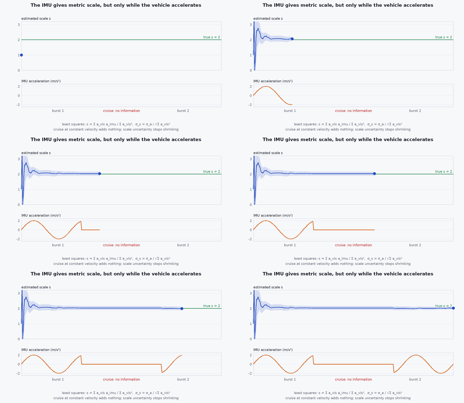
Scale: when the camera accelerates, the visual position (in arbitrary units) changes by an amount proportional to the true acceleration times the unknown scale; the accelerometer measures that same acceleration in metres. Compare them and the scale falls out, provided there is acceleration to see (constant-velocity motion does not excite scale). Gravity: the accelerometer always senses gravity, which fixes the down direction, so roll and pitch are observable; yaw and absolute position are not, because rotating or translating the entire world leaves every image and every inertial measurement unchanged.
Consequence: VIO drift is mostly in yaw and position; roll, pitch and scale are bounded. A global reference (GNSS, a map, a loop closure) is needed to bound the rest.
Mathematical formulation
The camera gives positions in arbitrary visual units, where is the metric position and the unknown scale (visual units per metre). The accelerometer, with gravity and bias removed, gives the metric world acceleration a = . The second difference of the visual position therefore satisfies a, and the scale follows by least squares:
The full VIO state in a filter or window is:
The observability argument (Hesch et al.; Kelly and Sukhatme) shows that the four unobservable directions must be respected by the estimator: filters that incorrectly gain information about yaw become inconsistent (overconfident), which is the motivation for observability-constrained filters such as OC-EKF and for the “first-estimate Jacobians” used in OpenVINS (lesson M3-T12).
- camera position from visual odometry in arbitrary units.
- metric scale factor (metres per visual unit).
- ,
- gyro and accelerometer biases.
Architecture and data flow
Inputs: stereo or monocular images with acquisition timestamps, IMU at high rate, camera–IMU extrinsics and time offset (calibration: lessons M7-T15 and M7-T16), IMU noise parameters (lesson M3-T7). Output: odometry and covariance in the odom frame, feature count and tracking quality for the monitor. Initialisation needs motion (to observe scale and gravity) and is a common failure point on the ground: arrange for a gentle initial movement. The output feeds PX4 EKF2 through the external vision interface (lesson M6-T10).
Real-world UAV applications
- GNSS-denied indoor and under-canopy flight.
- Visual position hold with metric scale.
- Front-end of Capstone 1.
- Providing high-rate pose for control between slower LiDAR updates.
Implementation example
This runs as shown: a vehicle accelerates sinusoidally; the camera observes position in arbitrary units (scale 0.37) with noise, the accelerometer measures true acceleration with bias; the least-squares estimate recovers the scale, and it fails (as expected) for constant-velocity motion.
import numpy as np
rng = np.random.default_rng(2)
dt, n = 0.05, 400; t = np.arange(n) * dt
s_true = 0.37                                                     # unknown scale: visual position = s_true * metric position (visual units per metre)

def run(accelerating=True):
    p = (np.stack([np.sin(0.8 * t), 0.5 * np.cos(0.5 * t), 0.2 * np.sin(1.3 * t)], axis=1) if accelerating else np.stack([2.0 * t, 0 * t, 0 * t], axis=1))
    a_true = np.gradient(np.gradient(p, dt, axis=0), dt, axis=0)                 # metric acceleration
    vis = s_true * p + 0.002 * rng.standard_normal(p.shape)                      # camera position in arbitrary units, with noise
    acc_meas = a_true + np.array([0.05, -0.03, 0.02]) + 0.02 * rng.standard_normal(p.shape)  # accelerometer with bias and noise
    vis_dd = np.gradient(np.gradient(vis, dt, axis=0), dt, axis=0)               # second difference of the visual position
    a = acc_meas - acc_meas.mean(axis=0) if not accelerating else acc_meas - np.array([0.05, -0.03, 0.02])   # bias known here; a real filter estimates it
    s_hat = np.sum(vis_dd * a) / np.sum(a * a)                                   # least squares: vis_dd = s * a
    return s_hat, np.sum(a * a)

s_hat, excitation = run(True)
print(f"scale: true {s_true}, estimated {s_hat:.3f}, excitation {excitation:.1f}")
assert abs(s_hat - s_true) < 0.03
s_const, exc_const = run(False)
print(f"constant velocity: excitation {exc_const:.2f}, 'estimated' scale {s_const:.2f}")
assert exc_const < 0.01 * excitation and abs(s_const - s_true) > 0.3 # no acceleration to compare: the scale estimate is noise (scale is unobservable)Common engineering mistakes
Initialising while stationary
Scale and gravity are unobservable without excitation: move gently at start.
Wrong camera–IMU time offset or extrinsics
The scale and biases absorb the error and drift appears in fast motion (lessons M7-T8, M7-T16).
Believing VIO bounds position
Yaw and position remain unobservable and drift.
Inflating IMU noise to hide inconsistency
It masks the root cause.
Ignoring tracking quality
The estimator needs to know when vision degrades.
Failure modes
| Failure mode | How it shows up | Likely cause |
|---|---|---|
| Scale drift | Trajectory size changes over time | Insufficient excitation or bad IMU noise parameters |
| Divergence after fast rotation | Estimate explodes | Motion blur, time offset, saturation |
| Initialisation failure | No estimate for several seconds | Stationary start, texture-poor scene |
| Yaw drift | Heading slowly rotates | Unobservable by construction without a global reference |
Debugging approach
- Plot the estimated scale (if estimated), gravity direction and biases against time.
- Record feature counts and compare with error growth.
- Run on a public dataset with ground truth before your own data.
- Check the camera–IMU calibration residuals.
Practical exercises
- Show that rotating the whole world about the vertical leaves the visual and inertial measurements unchanged.
- Compute the excitation needed for 5% scale accuracy under the given noise.
- Run VINS-Fusion or OpenVINS on EuRoC and report drift as a percentage of distance.
- List the four unobservable degrees of freedom and what could observe each.
Interview questions
Write an answer in your own words, then reveal the model answer. Nothing is sent anywhere.
Question 1
Why does adding an IMU fix monocular scale?
Model answer
The accelerometer measures metric acceleration; comparing it with the visual second difference during accelerating motion gives the scale factor.
Question 2
What is unobservable in VIO?
Model answer
Global position and yaw (four degrees of freedom): shifting or rotating the world about gravity changes no measurement, so these drift.
Question 3
What is the difference between MSCKF and sliding-window VIO?
Model answer
MSCKF is a filter that marginalises features and updates with constraints between past camera poses; sliding-window systems optimise keyframe states and features jointly with IMU preintegration factors.
References and further reading
Primary papers, official documentation and standards. Each claim above that is specific to a tool or version points here.
- A. Mourikis, S. Roumeliotis, “A multi-state constraint Kalman filter for vision-aided inertial navigation”, ICRA 2007
- T. Qin, P. Li, S. Shen, “VINS-Mono”, arXiv:1708.03852
- P. Geneva et al., “OpenVINS: a research platform for visual-inertial estimation”, ICRA 2020
- C. Forster et al., “On-manifold preintegration for real-time visual-inertial odometry”, IEEE T-RO, 2017
- J. A. Hesch, D. G. Kottas, S. L. Bowman, S. I. Roumeliotis, “Camera-IMU-based localization: observability analysis and consistency improvement”, IJRR, 2014