UAV Systems Engineering · Module 2
M2-T10: Visual Odometry
Two images of a static scene constrain how the camera moved between them, up to an unknown scale: derive the geometry, run it, and see why it drifts.
A camera is a cheap, light, information-rich sensor, and the geometry of how images change as a camera moves is exact. Visual odometry turns that geometry into a motion estimate, and the same geometry explains where it fails.
Learning objectives
After this lesson, you should be able to:
- Describe the stages of a feature-based visual odometry pipeline.
- State the epipolar constraint and the essential matrix, and recover and from it.
- Explain why monocular translation has an unknown scale and how stereo or an IMU resolves it.
- Name the main failure modes and the inlier statistics that reveal them.
Conceptual explanation
Visual odometry (VO) estimates the camera’s motion by tracking how image content moves. A feature-based pipeline detects distinctive points (corners), matches them between consecutive frames, rejects wrong matches with RANSAC, estimates the relative pose between the frames, and composes those relative poses into a trajectory.
Because each step estimates the motion relative to the previous frame, errors accumulate: VO is dead reckoning with a camera and drifts, typically as a small percentage of distance travelled when it works well.
Engineering intuition
For a camera that translates, nearby points move a lot in the image and distant points move little (parallax). For a camera that rotates, all points shift together regardless of depth. Parallax therefore carries the translation, and uniform image shifts carry the rotation. Without parallax (a distant scene, a pure rotation) the translation is unobservable, and VO degenerates.
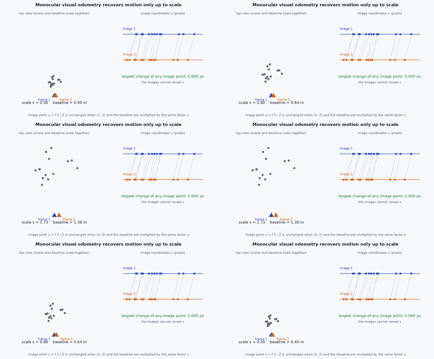
A single camera sees only bearings, not distances, so it can tell you the direction of motion but not how far it went: doubling the scene and the motion gives identical images. That unknown scale is the central weakness of monocular VO and the main reason a UAV adds an IMU, a stereo pair or a rangefinder.
Mathematical formulation
For corresponding points , (homogeneous, in normalised camera coordinates, applied to pixels), the two views satisfy the epipolar constraint:
- ,
- normalised image coordinates of the same 3-D point in the first and second camera.
- ,
- rotation and translation taking points from the first camera frame to the second: .
- [t]ₓ
- skew-symmetric matrix of , so [t]ₓ v = t × v.
- essential matrix: rank 2 with two equal singular values and one zero.
The constraint is linear in the nine entries of , so five points suffice with the minimal solver (Nistér) and eight with the classical eight-point algorithm: stack the equations, take the singular vector of the smallest singular value, and enforce the rank-2 / equal-singular-values structure. Decompose with the SVD, :
The translation is recovered only up to scale: is unchanged if is multiplied by a constant. Stereo (known baseline), an IMU (metric acceleration) or a known altitude fixes the scale.
RANSAC
Repeatedly sample a minimal set of matches, fit , count matches with small epipolar error (inliers), and keep the model with most inliers. The number of iterations needed is for a desired success probability , outlier fraction and sample size : for , , this is about 146.
Architecture and data flow
Camera (hardware-timestamped frames) → front-end (detect, track) → relative-pose solver → pose and covariance → fusion (lesson M3-T9). The front-end’s health metrics (feature count, inlier ratio, parallax) must be published with the pose so a monitor can lower confidence before the estimate fails (lesson M8-T12).
Real-world UAV applications
- GNSS-denied navigation indoors, under canopy and in urban canyons.
- Optical-flow-based velocity for position hold (a simplified VO).
- Front-end of VIO and visual SLAM systems (ORB-SLAM3, VINS-Fusion, OpenVINS).
- Landing on moving platforms and relative navigation near structures.
Implementation example
This runs as shown: it creates a synthetic scene and camera motion, estimates with the eight-point algorithm, decomposes it, and verifies that the rotation is recovered exactly and the translation direction matches (the length is lost).
import numpy as np
rng = np.random.default_rng(0)

def rodrigues(w):
    th = np.linalg.norm(w)
    if th < 1e-12: return np.eye(3)
    k = w / th; K = np.array([[0, -k[2], k[1]], [k[2], 0, -k[0]], [-k[1], k[0], 0]])
    return np.eye(3) + np.sin(th) * K + (1 - np.cos(th)) * K @ K

X = rng.uniform([-4, -3, 6], [4, 3, 14], size=(60, 3))      # 3-D points in front of camera 1
R_true = rodrigues(np.array([0.02, -0.05, 0.03]))
t_true = np.array([0.8, 0.1, 0.2])                         # metres: scale is arbitrary
X2 = X @ R_true.T + t_true
x1 = X[:, :2] / X[:, 2:3]; x2 = X2[:, :2] / X2[:, 2:3]       # normalised image coordinates
x1 += 1e-4 * rng.standard_normal(x1.shape); x2 += 1e-4 * rng.standard_normal(x2.shape)   # pixel noise at f ~ 700 px

def eight_point(a, b):
    A = np.array([[bx*ax, bx*ay, bx, by*ax, by*ay, by, ax, ay, 1] for (ax, ay), (bx, by) in zip(a, b)])
    E = np.linalg.svd(A)[2][-1].reshape(3, 3)
    U, _, Vt = np.linalg.svd(E)
    return U @ np.diag([1, 1, 0]) @ Vt                      # enforce the essential-matrix structure

E = eight_point(x1, x2)

def decompose(E):
    U, _, Vt = np.linalg.svd(E)
    if np.linalg.det(U) < 0: U = -U
    if np.linalg.det(Vt) < 0: Vt = -Vt
    W = np.array([[0, -1, 0], [1, 0, 0], [0, 0, 1.0]])
    return [(U @ W @ Vt, U[:, 2]), (U @ W @ Vt, -U[:, 2]), (U @ W.T @ Vt, U[:, 2]), (U @ W.T @ Vt, -U[:, 2])]

def in_front(R, t, a, b):
    count = 0
    for (ax, ay), (bx, by) in zip(a, b):                    # triangulate by least squares: depth along ray 1
        r1 = np.array([ax, ay, 1.0]); r2 = np.array([bx, by, 1.0])
        M = np.stack([R @ r1, -r2], axis=1)
        s, *_ = np.linalg.lstsq(M, -t, rcond=None)
        count += (s[0] > 0) and (s[1] > 0)
    return count

best = max(decompose(E), key=lambda c: in_front(c[0], c[1], x1, x2))
R_est, t_est = best
ang = np.degrees(np.arccos(np.clip((np.trace(R_est.T @ R_true) - 1) / 2, -1, 1)))
cos_t = t_est @ t_true / np.linalg.norm(t_true)
print(f"rotation error {ang:.4f} deg, translation direction cosine {cos_t:.5f}  (length lost: |t_est| = {np.linalg.norm(t_est):.2f}, true {np.linalg.norm(t_true):.2f})")
assert ang < 0.2 and cos_t > 0.995Common engineering mistakes
Assuming the monocular translation has metric length
The scale is arbitrary; metric scale needs stereo, an IMU, an altitude or a known object.
Estimating E for a nearly planar or distant scene
Planar scenes give a degenerate : use a homography. A scene with no parallax gives no translation information.
Skipping RANSAC or using too few iterations
A few wrong matches can dominate a least-squares fit.
Not publishing front-end health
The downstream filter cannot lower its trust when tracking degrades.
Using a rolling-shutter camera with global-shutter geometry
Fast motion bends straight lines and biases rotation. Model it or use a global shutter.
Failure modes
| Failure mode | How it shows up | Likely cause |
|---|---|---|
| Low texture | Feature count and inliers collapse; pose freezes or jumps | White walls, water, uniform grass, fog |
| Motion blur or exposure change | Features vanish during aggressive manoeuvres or sun transitions | Exposure time too long, auto-exposure lag |
| Dynamic scene | Inliers cluster on a moving object; estimate follows it | Crowds, vehicles, foliage in wind |
| Pure rotation or no parallax | Translation estimate is noisy or wrong while rotation is fine | Hovering rotation, distant scenes |
| Scale drift | Trajectory shape is right but its size changes over time | Monocular scale is not constrained |
Debugging approach
- Plot feature count, inlier ratio and median parallax over time: failures are visible there before they appear in the pose.
- Overlay tracked features on the image to see whether they sit on the static scene.
- Test on a dataset with ground truth first (TUM-VI, EuRoC) and measure drift as a percentage of distance with an evaluation tool such as evo.
- Check exposure and frame timestamps: dropped or irregular frames break constant-motion assumptions.
Practical exercises
- Compute the number of RANSAC iterations for the five-point solver with 70% outliers and 99.9% confidence.
- Add 20% random wrong matches to the code example and compare the eight-point fit with and without RANSAC.
- Show that scaling and all 3-D points by 2 leaves the images unchanged.
- Use the Visual Odometry Simulator to find the texture density at which tracking is lost at 3 m/s.
Interview questions
Write an answer in your own words, then reveal the model answer. Nothing is sent anywhere.
Question 1
Why can monocular VO not recover metric scale?
Model answer
Images are unchanged if the scene and translation are scaled together, so the epipolar constraint determines translation only up to scale. Scale needs extra information: stereo baseline, IMU accelerations, known altitude or object size.
Question 2
What is the essential matrix and what does it encode?
Model answer
ₓ relates normalised image points in two views by Ex = 0. It encodes relative rotation and translation direction between two calibrated cameras.
Question 3
Why is RANSAC used?
Model answer
Matches contain outliers that destroy least-squares fits. RANSAC finds the model supported by the largest consistent set by sampling minimal subsets, tolerating a large fraction of wrong matches.
References and further reading
Primary papers, official documentation and standards. Each claim above that is specific to a tool or version points here.
- D. Scaramuzza, F. Fraundorfer, “Visual odometry [tutorial]”, IEEE RAM, 2011
- D. Nistér, “An efficient solution to the five-point relative pose problem”, IEEE TPAMI, 2004
- M. Fischler, R. Bolles, “Random sample consensus”, Communications of the ACM, 1981
- OpenCV: epipolar geometry tutorial
- . Hartley, A. Zisserman, Multiple View Geometry in Computer Vision, 2nd ed., Cambridge University Press, 2004.