UAV Systems Engineering · Module 4
M4-T8: FAST-LIO2
FAST-LIO2 registers raw LiDAR points straight against an incrementally updated map inside an iterated Kalman filter: the idea, the maths and a toy version you can run.
FAST-LIO2 is among the most widely used open-source LiDAR-inertial odometry systems for UAVs and it is the engine of Capstone 2. This lesson explains how it works, using a small runnable example of its central operation, and states clearly what it can and cannot do.
Learning objectives
After this lesson, you should be able to:
- Describe the FAST-LIO2 pipeline: propagation, undistortion, iterated update and incremental map.
- Explain the iterated Kalman filter update and why iterating helps for scan registration.
- Write the point-to-plane residual used for registration.
- List the assumptions and failure modes: degenerate geometry, dynamic scenes, IMU extrinsics, time sync.
Conceptual explanation
Research-level This is a description of a published research system (Xu et al., IEEE T-RO 2022) and its open-source implementation. Behaviour depends on the sensor, scene, configuration and software version; consult the repository and the paper.
FAST-LIO2 is a tightly coupled LiDAR-inertial odometry method. Three ideas distinguish it:
- Direct registration: it uses the raw points of each scan (after downsampling) rather than extracting edge and plane features as LOAM does, so no feature extractor has to be tuned for each LiDAR.
- Iterated extended Kalman filter on a manifold state (pose, velocity, IMU biases, gravity, optionally LiDAR-IMU extrinsics): scan registration residuals are the measurements.
- ikd-Tree: an incremental k-d tree that supports point insertion, deletion and dynamic re-balancing, so the map can be updated every scan and nearest-neighbour searches stay fast.
Because a scanning LiDAR collects points over about 0.1 s while the vehicle moves, each point is measured at a slightly different pose. FAST-LIO2 back-propagates through the IMU-predicted poses to express every point in the frame at the end of the scan (undistortion), which is essential at UAV speeds.
Engineering intuition
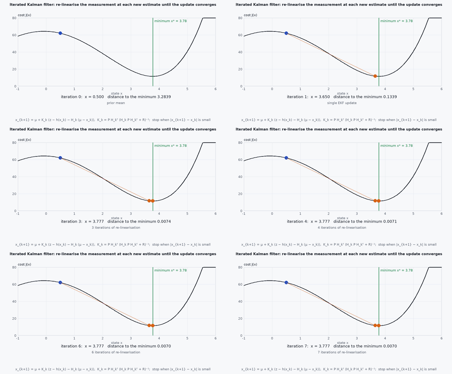
Picture overlaying the new scan on the map you have built. If the IMU prediction is good the overlay is nearly right, and the filter nudges the state until points sit on the surfaces they hit. Because the relation between pose and residual is nonlinear, one linearised step lands close but not exactly; iterating (relinearising at each improved estimate while keeping the prior from the IMU) walks into the right answer. The prior from the IMU is the guard rail: it stops the update from sliding along a surface it cannot see, and when the geometry is degenerate (a long corridor), the covariance reflects that the along-corridor position is unconstrained and the result drifts there.
Mathematical formulation
State on a manifold (rotation in SO(3)); IMU propagation gives the prior with covariance . For each downsampled point in the LiDAR frame, the world point is , and the point-to-plane residual is the distance to the plane fitted to its nearest map neighbours (unit normal , a point on the plane):
The measurement model is plus noise; the iterated update repeats, with the Jacobian of at the current iterate :
- ⊞, ⊟
- addition and subtraction on the state manifold (rotations handled on SO(3)).
- ,
- prior from IMU propagation.
- measurement noise of the residuals, set by LiDAR range noise.
- (x),
- stacked point-to-plane residuals and their Jacobian with respect to the state error.
This is the MAP estimate of the state given the prior and the residuals, found by Gauss–Newton: the iteration is the optimisation, and the final ⁺ is the Laplace approximation of the posterior covariance. One important efficiency fact from the paper: with hundreds or thousands of residuals the gain can be computed in the state dimension rather than the measurement dimension, which is what makes the update fast.
Architecture and data flow
Inputs: LiDAR point cloud with per-point time (for undistortion), IMU at its native rate, and the LiDAR-IMU extrinsics (rotation and translation) as configuration. Outputs: odometry (pose, velocity) at the LiDAR rate with covariance, the registered point cloud and the accumulated map. The state can feed the PX4 external-odometry bridge (lesson M6-T10) after frame conversion and timestamp handling. Time synchronisation between IMU and LiDAR is a precondition (lesson M7-T8): a few milliseconds of offset visibly smear the map during rotation.
Real-world UAV applications
- GNSS-denied UAV navigation and mapping in tunnels, forests, warehouses and around structures.
- High-speed flight with a solid-state or spinning LiDAR and an IMU.
- Real-time 3-D map building for inspection.
- The odometry front-end of FAST-LIVO2 and other LiDAR-inertial-visual systems (lesson M4-T10).
Implementation example
This runs as shown: a toy planar version of the central operation. A scan taken inside a square room is registered against the room’s walls by an iterated Kalman update from a wrong prior. It shows why iterating helps, and that the posterior is far better than the prior. It is a 2-D teaching model, not the FAST-LIO2 code.
import numpy as np
rng = np.random.default_rng(2)
walls = [(np.array([0, 1.0]), 5.0), (np.array([0, -1.0]), 5.0), (np.array([1.0, 0]), 5.0), (np.array([-1.0, 0]), 5.0)]   # n . q = d (10 m room)
R2 = lambda t: np.array([[np.cos(t), -np.sin(t)], [np.sin(t), np.cos(t)]])
dR2 = lambda t: np.array([[-np.sin(t), -np.cos(t)], [np.cos(t), -np.sin(t)]])

true = np.array([0.5, -0.4, 0.2])                                 # x, y, heading: the pose to recover
pts = []
for a in np.linspace(0, 2 * np.pi, 180, endpoint=False):          # simulate a 360-degree scan from the true pose
    dw = R2(true[2]) @ np.array([np.cos(a), np.sin(a)]); best = 1e9
    for n, d in walls:
        den = n @ dw
        if den > 1e-6: lam = (d - n @ true[:2]) / den; best = min(best, lam) if lam > 0 else best
    pts.append(R2(true[2]).T @ (best * dw) + 0.02 * rng.standard_normal(2))      # point in the sensor frame + 2 cm noise
pts = np.array(pts)

def residuals(x):                                                   # point-to-plane residuals r_j and Jacobian rows
    r, H = [], []
    for p in pts:
        q = R2(x[2]) @ p + x[:2]
        n, d = min(walls, key=lambda w: abs(w[0] @ q - w[1]))      # nearest plane = data association
        r.append(n @ q - d); H.append(np.concatenate([n, [n @ (dR2(x[2]) @ p)]]))
    return np.array(r), np.array(H)

xbar = true + np.array([0.3, -0.2, 0.1])                           # IMU-propagated prior: 36 cm and 5.7 deg off
P = np.diag([0.5**2, 0.5**2, 0.2**2]); Rn = 0.05**2

def iterated_update(xbar, P, iters):
    x = xbar.copy()
    for _ in range(iters):
        r, H = residuals(x)
        K = P @ H.T @ np.linalg.inv(H @ P @ H.T + Rn * np.eye(len(r)))
        x = xbar + K @ (-r - H @ (xbar - x))                        # relinearise at x, keep the prior at xbar
    return x

for iters in (1, 2, 5):
    x = iterated_update(xbar, P, iters)
    print(f"{iters} iteration(s): position error {1000 * np.linalg.norm(x[:2] - true[:2]):.1f} mm, heading error {np.degrees(abs(x[2] - true[2])):.3f} deg")
e1 = np.linalg.norm(iterated_update(xbar, P, 1)[:2] - true[:2]); e5 = np.linalg.norm(iterated_update(xbar, P, 5)[:2] - true[:2])
assert e5 < e1 < 0.05 and e5 < 0.01 and np.linalg.norm(xbar[:2] - true[:2]) > 0.3Common engineering mistakes
Wrong LiDAR-IMU extrinsics
Systematic drift and smeared maps. Calibrate (lesson M7-T16) or let the filter estimate them with a good initial guess.
Unsynchronised IMU and LiDAR clocks
A few ms of offset blur the map during rotation; fix timestamps first.
Assuming it works in any scene
Long corridors, open fields and tunnels have degenerate geometry; add other aiding (vision, barometer, GNSS when present).
Ignoring dynamic objects
Moving people and vehicles bias registration; downsample and filter, and monitor residuals.
Using default parameters for a different LiDAR
Check scan period, point-time field, blind distance and downsampling for your sensor in the configuration.
Failure modes
| Failure mode | How it shows up | Likely cause |
|---|---|---|
| Degeneracy | Drift along a corridor axis while covariance stays small | Geometry does not constrain one direction |
| Map smearing during turns | Double walls in the accumulated map | Time offset or wrong extrinsic rotation |
| Divergence under vibration or aggressive flight | Pose jumps or runs away | IMU saturation or noise parameters wrong |
| Slow processing | Latency rises as the map grows | Map size or downsampling not constrained for the compute budget |
Debugging approach
- Record a bag and view the accumulated point cloud: double surfaces reveal extrinsic or timing errors.
- Plot the registration residual (and the number of effective points) over time: sudden loss of points or rising residual flags degeneracy.
- Evaluate against ground truth with evo for ATE and RPE on a public dataset first.
- Profile CPU use and per-scan latency on the target computer (module 7).
Practical exercises
- Show that with the prior covariance very large (uninformative), the iterated update reduces to Gauss–Newton ICP.
- Run the toy example in a long corridor (remove the end walls) and compute the uncertainty along its axis.
- Add a 5 ms timing error to the toy scan with rotation and measure the error it causes.
- Read the FAST-LIO2 configuration for your LiDAR and list the parameters that must match the hardware.
Interview questions
Write an answer in your own words, then reveal the model answer. Nothing is sent anywhere.
Question 1
What is the key difference between LOAM and FAST-LIO2 in the way they use LiDAR points?
Model answer
LOAM extracts edge and planar features and registers those; FAST-LIO2 registers the raw (downsampled) points directly against the map, which avoids feature extraction and works across LiDAR types.
Question 2
Why does an iterated Kalman filter help in scan registration?
Model answer
The residual is nonlinear in pose; a single linearised update can be inaccurate. Iterating relinearises at improved estimates while keeping the IMU prior, converging to the MAP solution.
Question 3
When will FAST-LIO2 drift without any sign of failure?
Model answer
In geometrically degenerate scenes such as long corridors or open fields, where the scan does not constrain motion along some direction; other sensors or global references are needed.
References and further reading
Primary papers, official documentation and standards. Each claim above that is specific to a tool or version points here.
- W. Xu, Y. Cai, D. He, J. Lin, F. Zhang, “FAST-LIO2: Fast direct LiDAR-inertial odometry”, IEEE T-RO, 2022
- FAST-LIO2 on arXiv:2107.06829
- W. Xu, F. Zhang, “FAST-LIO: A fast, robust LiDAR-inertial odometry package by tightly-coupled iterated Kalman filter”, arXiv:2010.08196
- Y. Cai, W. Xu, F. Zhang, “ikd-Tree: an incremental k-d tree for robotic applications”, arXiv:2102.10808
- FAST-LIO repository (includes FAST-LIO2 code)