UAV Systems Engineering · Module 4
M4-T7: LOAM and A-LOAM
LOAM’s insight was to split the problem by rate: fast and rough scan-to-scan odometry, slow and precise scan-to-map mapping, with sharp edges and flat surfaces as features.
LOAM (Zhang and Singh, RSS 2014) set the pattern for feature-based LiDAR SLAM and A-LOAM is a widely used open implementation. Its core is a simple local-geometry measure: the smoothness (curvature) of points along a scan line.
Learning objectives
After this lesson, you should be able to:
- Compute the LOAM smoothness measure and classify edge and planar points.
- Describe the two-rate structure: odometry and mapping.
- Explain point-to-edge and point-to-plane residuals.
- State what A-LOAM is and its dependence on the LiDAR scan pattern.
Conceptual explanation
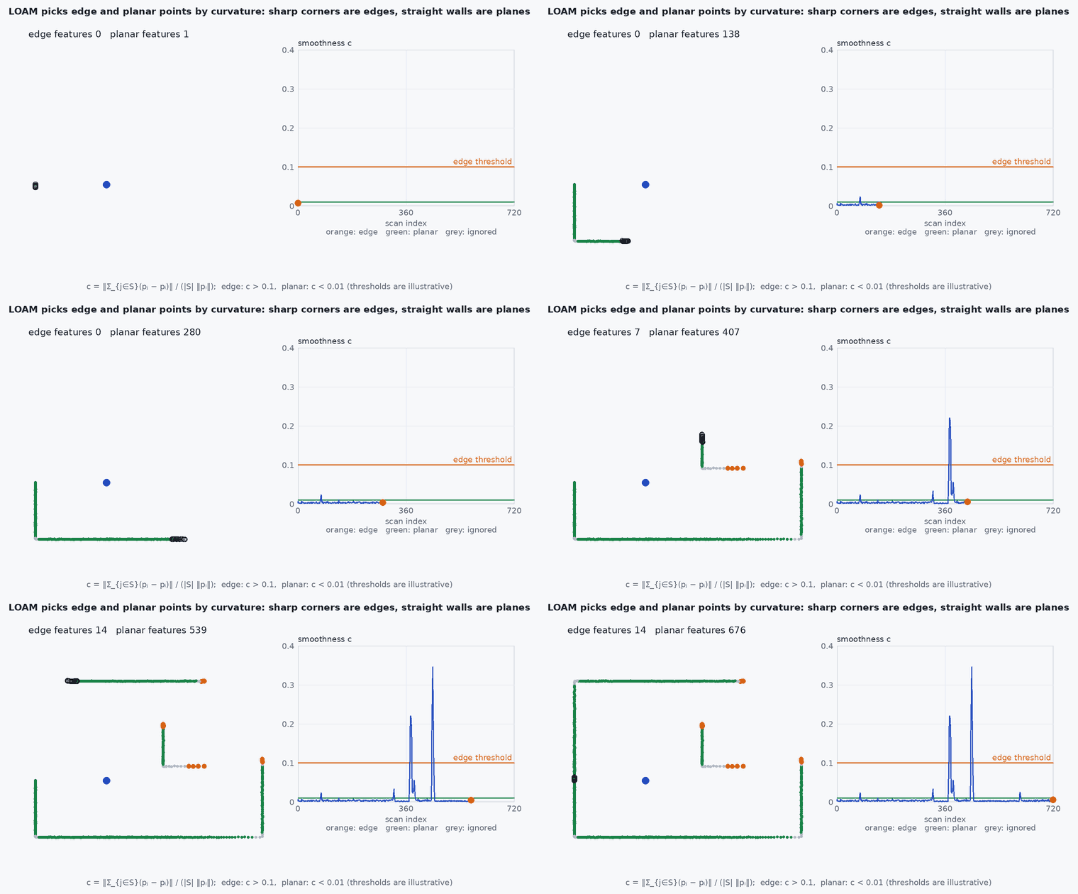
Along each scan line of a spinning LiDAR, LOAM computes a local curvature for each point from its neighbours. Points with large are edge features (corners), points with small are planar features (flat surfaces). Registration minimises distances from edge points to edge lines and from planar points to planar patches in the previous scan (odometry, ~10 Hz) and then in an accumulated map (mapping, ~1 Hz, more precise). The original LOAM uses a constant-velocity assumption within a scan for distortion; A-LOAM (an “advanced” re-implementation by Qin and Cao) uses Ceres and Eigen, dropping the IMU.
Engineering intuition
An edge is where a surface turns sharply: a point there differs strongly from the average of its neighbours; a plane has neighbours that average back onto the point. Both features constrain the pose differently: planes constrain along their normal (lesson M2-T13), edges constrain across the line. Using both gives constraints in more directions than planes alone. The split into odometry and mapping uses the fact that a good initial guess (from the previous scan) makes the expensive scan-to-map step converge quickly at a low rate.
Mathematical formulation
For point on a scan line with the set of neighbouring points on each side (typically five on each side) and range vectors , the smoothness is:
Selection rules in the paper also exclude points near occlusion boundaries and nearly parallel to the beam. Residuals: for an edge point and the line through two map edge points a and , ; for a planar point and a plane through three points, . The pose is found by Levenberg–Marquardt on the sum of squared distances (lesson M2-T14 for the ICP analogue).
- neighbourhood on the same scan line.
- threshold, a tuning parameter for each LiDAR.
- a, ,
- map points defining the edge line or the plane.
Architecture and data flow
A-LOAM expects a spinning multi-line LiDAR point cloud with a known number of scan lines (the feature extraction uses the ring structure) and publishes odometry and a map; it does not use an IMU, so it will distort under fast motion where an IMU-aided method will not (lesson M3-T10). Solid-state LiDARs with irregular scan patterns need different feature handling (this is why FAST-LIO’s direct approach is popular on them). Check the README of the repository for the topics and parameters (scan_line, mapping_line_resolution, mapping_plane_resolution).
Real-world UAV applications
- Baseline LiDAR odometry and mapping with a spinning LiDAR.
- Teaching feature-based registration.
- Comparing against FAST-LIO2 on the same data.
- Feature extraction as the front-end of LeGO-LOAM and LIO-SAM.
Implementation example
This runs as shown: LOAM smoothness on a synthetic scan line crossing a wall corner: the corner point is detected as an edge and points on the flat walls as planar.
import numpy as np

def smoothness(X, half=5):
    n = len(X); c = np.full(n, np.nan)
    for i in range(half, n - half):
        nb = [j for j in range(i - half, i + half + 1) if j != i]
        c[i] = np.linalg.norm(np.sum(X[i] - X[nb], axis=0)) / (2 * half * np.linalg.norm(X[i]))
    return c

# one scan line in the horizontal plane: the sensor at the origin sees two walls meeting at a corner (x = 6 and y = 4)
angles = np.radians(np.linspace(-20, 55, 150)); pts = []
for a in angles:
    d = np.array([np.cos(a), np.sin(a)]); r_x = 6.0 / d[0]; r_y = 4.0 / d[1] if d[1] > 1e-6 else 1e9
    pts.append(min(r_x, r_y) * d)
X = np.array(pts) + 0.002 * np.random.default_rng(0).standard_normal((150, 2))
c = smoothness(X)
corner = int(np.nanargmax(c)); thr = 0.01
edges = np.where(c > thr)[0]; planar = np.where(c < 0.002)[0]
corner_true = int(np.argmin(np.abs(np.arctan2(4.0, 6.0) - angles)))
print(f"corner at index {corner_true}; max curvature at {corner} (c = {c[corner]:.3f}); {len(edges)} edge-candidate and {len(planar)} planar points")
assert abs(corner - corner_true) <= 2 and c[corner] > 0.015
assert len(planar) > 80 and len(edges) < 15 and np.all(np.abs(edges - corner_true) <= 7)Common engineering mistakes
Using A-LOAM on a solid-state LiDAR without adapting the feature extraction
It assumes ring structure.
No IMU on a fast UAV
Scan distortion degrades the result (lesson M3-T10).
Thresholds copied between sensors
Curvature scale depends on resolution and range noise.
Evaluating on a flat scene
Few edge features: the pose is poorly constrained.
Expecting loop closure from LOAM itself
It is odometry and mapping; add a loop-closure back-end.
Failure modes
| Failure mode | How it shows up | Likely cause |
|---|---|---|
| Drift in corridors | Along-axis drift | Planes only constrain across the corridor |
| Smeared map on fast turns | Ghost surfaces | No IMU for deskewing |
| Feature starvation | Odometry jumps in featureless areas | Too few edges or planes |
| High latency | Slow mapping thread | Map resolution too fine for the CPU |
Debugging approach
- Visualise the extracted edge and planar points on a scan.
- Check scan-line count and ring ordering of your driver.
- Evaluate with evo and compare with a LIO method on the same bag.
- Profile the mapping thread.
Practical exercises
- Tune the threshold on a synthetic scan line with sharper and shallower corners.
- Derive the point-to-line distance and its Jacobian.
- Run A-LOAM on a public dataset and report drift as a percentage of distance.
- Explain why the mapping step runs at a lower rate than the odometry step.
Interview questions
Write an answer in your own words, then reveal the model answer. Nothing is sent anywhere.
Question 1
How does LOAM decide edge and planar points?
Model answer
By the smoothness (curvature) of points along a scan line computed from neighbouring points: high curvature is an edge, low is planar.
Question 2
Why does LOAM have two rates?
Model answer
Scan-to-scan odometry is fast and approximate; scan-to-map mapping is slower but more accurate, and benefits from the odometry initial guess.
Question 3
What is A-LOAM?
Model answer
An open-source “advanced” implementation of LOAM using Ceres and Eigen without an IMU, popular as a baseline.
References and further reading
Primary papers, official documentation and standards. Each claim above that is specific to a tool or version points here.