UAV Systems Engineering · Module 4
M4-T6: LiDAR SLAM
LiDAR SLAM turns scans into a metric map; the design choices are what to register (features or raw points), what to store (voxels or points) and how to close loops.
LiDAR gives direct 3-D geometry, so LiDAR SLAM systems tend to be metrically accurate and robust to lighting. The families differ in how they register scans and how they store the map, and those choices set their speed, robustness and failure modes.
Learning objectives
After this lesson, you should be able to:
- Compare feature-based (LOAM family) and direct (FAST-LIO family) registration.
- Describe map representations and the role of voxel downsampling.
- Explain loop closure with global scan descriptors.
- Choose a LiDAR SLAM approach for a UAV and state its limits.
Conceptual explanation
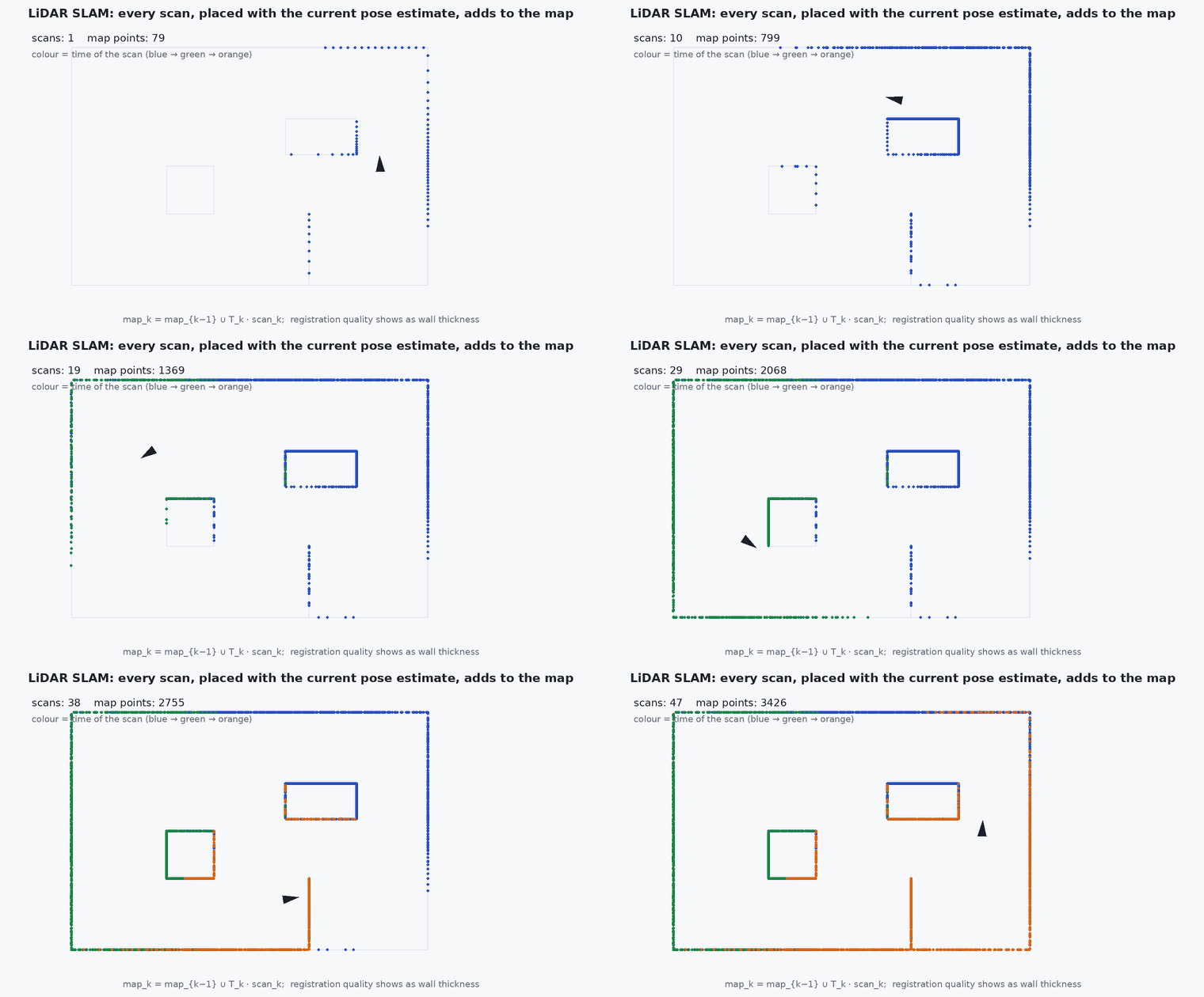
Feature-based methods (LOAM, A-LOAM, LeGO-LOAM) extract edge and planar points by local curvature and register them to a feature map (lesson M4-T7). Direct methods (FAST-LIO, FAST-LIO2, KISS-ICP) register downsampled raw points to a point or voxel map, without feature extraction (lesson M4-T8). Both fuse an IMU for deskewing and prediction. Back-ends add loop closure and pose-graph optimisation (LIO-SAM, LeGO-LOAM with SC).
Engineering intuition
A raw LiDAR frame holds tens of thousands of points; registering them all is unnecessary and expensive. A voxel filter keeps one representative per cell, giving even density and bounded cost. Feature extraction is a second kind of filtering that keeps only informative points (edges and planes), but needs tuning for each LiDAR’s scan pattern; direct methods skip it and accept more points. For loop closure, a global descriptor of a scan (for example a polar height map, as in Scan Context) lets a place be recognised from a different heading without any prior pose.
Mathematical formulation
Voxel downsampling: points with voxel size fall in cell ; replace each occupied cell by the centroid (or the point closest to it). The number of retained points is bounded by the occupied volume divided by , independent of the raw point count. Registration cost is then proportional to the retained points times the neighbour-search cost (lesson M2-T14).
Scan Context-style loop closure: encode the scan as a matrix of maximum heights over (ring, sector) bins; compare two descriptors by the column-shifted distance (to be yaw-invariant), then verify with ICP. Pose-graph optimisation (lesson M4-T12) distributes the loop correction. Map size must be bounded (sliding local map, keyframe submaps) for constant compute.
- voxel edge length (m): 0.1–0.5 m is typical in published systems for indoor to outdoor scenes (a tuning choice).
- number of points in voxel .
Architecture and data flow
Hardware: LiDAR (rotating or solid-state), IMU, calibrated extrinsics, shared clock. Software: LIO node → odometry and local map; back-end → global map and pose graph; output frames: odom (smooth) and map (corrected). Choose the algorithm using the LiDAR’s field of view (solid-state LiDARs with a narrow field favour direct methods), the scene geometry (corridors need degeneracy handling, lesson M2-T13) and the compute budget (lesson M7-T12).
Real-world UAV applications
- GNSS-denied mapping and localisation (Capstone 2).
- Building prior maps for map-based localisation (lesson M4-T13).
- Obstacle maps for planning.
- Inspection with repeatable localisation.
Implementation example
This runs as shown: a voxel-grid filter on a dense synthetic cloud: the point count falls by an order of magnitude while the shape (centroid and extent) is preserved, and the retained count tracks the occupied volume, not the raw density.
import numpy as np
rng = np.random.default_rng(1)

def voxel_filter(P, v):
    cells = np.floor(P / v).astype(np.int64)
    _, inv, counts = np.unique(cells, axis=0, return_inverse=True, return_counts=True)
    sums = np.zeros((counts.size, 3)); np.add.at(sums, inv.ravel(), P)
    return sums / counts[:, None]

# a dense cloud on three walls of a 10 x 8 x 3 m room (about 90 000 points)
def wall(n, axis, value, ext):
    P = np.stack([rng.uniform(0, ext[0], n), rng.uniform(0, ext[1], n), rng.uniform(0, ext[2], n)], axis=1); P[:, axis] = value; return P
P = np.vstack([wall(40000, 0, 0.0, (0, 8, 3)), wall(40000, 1, 0.0, (10, 0, 3)), wall(10000, 2, 0.0, (10, 8, 0))]) + 0.005 * rng.standard_normal((90000, 3))
for v in (0.1, 0.25, 0.5):
    Q = voxel_filter(P, v); print(f"voxel {v} m: {len(P)} -> {len(Q)} points ({100 * len(Q) / len(P):.1f}%)")
Q = voxel_filter(P, 0.25)
assert len(Q) < len(P) / 10 and np.allclose(Q.min(0), P.min(0), atol=0.3) and np.allclose(Q.max(0), P.max(0), atol=0.3)
assert len(voxel_filter(np.vstack([P, P + 0.001]), 0.25)) <= len(Q) + 100 # doubling the density barely changes the retained count: bounded costCommon engineering mistakes
No downsampling
Registration cost explodes and gives no accuracy benefit.
Voxel size not matched to the scene
Too large loses structure, too small keeps cost; tune per environment.
Unbounded global map in the odometry loop
Use a local sliding map for registration.
No loop closure verification
Aliasing in repeated structure causes false loops.
Treating the corrected map-frame pose as continuous
Use odom for control.
Failure modes
| Failure mode | How it shows up | Likely cause |
|---|---|---|
| Corridor drift | Along-axis drift | Degenerate geometry (lesson M2-T13) |
| Map smear | Double walls | Timing, extrinsics |
| Dynamic objects | Ghost objects in the map | No dynamic filtering |
| Compute overrun | Latency growth | Map or point count unbounded |
Debugging approach
- Look at the map for double surfaces and scale drift.
- Plot the points per scan after filtering and the registration time.
- Evaluate drift with evo against ground truth.
- Check loop-closure accept/reject statistics.
Practical exercises
- Estimate the retained points for a floor at 0.25 m voxels.
- Compare feature-based and direct registration in terms of tuning parameters.
- Choose a LiDAR SLAM method for a solid-state LiDAR with a field of view and justify it.
- Describe how Scan Context achieves yaw invariance.
Interview questions
Write an answer in your own words, then reveal the model answer. Nothing is sent anywhere.
Question 1
What is the difference between LOAM and FAST-LIO style registration?
Model answer
LOAM extracts edge and planar features and registers them; FAST-LIO registers downsampled raw points directly to a map, avoiding feature extraction.
Question 2
Why voxel-filter the scan?
Model answer
It bounds the point count and gives uniform density so the registration cost is predictable and accuracy is unharmed.
Question 3
How does a global scan descriptor help loop closure?
Model answer
It encodes the scan in a way that is comparable across viewpoints and headings, proposing candidates that are then verified geometrically.
References and further reading
Primary papers, official documentation and standards. Each claim above that is specific to a tool or version points here.
- T. Shan et al., “LIO-SAM: tightly-coupled lidar inertial odometry via smoothing and mapping”, IROS 2020
- G. Kim, A. Kim, “Scan Context: egocentric spatial descriptor for place recognition within 3D point cloud map”, IROS 2018
- W. Xu et al., “FAST-LIO2”, IEEE T-RO, 2022
- KISS-ICP: a simple, robust point-to-point LiDAR odometry pipeline (repository and paper link)