UAV Systems Engineering · Module 4
M4-T5: OpenVINS
OpenVINS keeps features out of the state with a linear-algebra trick: project the residual into the null space of the feature Jacobian.
OpenVINS (Geneva et al., ICRA 2020) is an open research platform built on the multi-state constraint Kalman filter. It is a filter where optimisation-based systems use a window, and its design choices (null-space elimination, first-estimate Jacobians, online calibration) explain its behaviour and its documentation.
Learning objectives
After this lesson, you should be able to:
- Describe the MSCKF structure: a window of cloned camera poses and features eliminated by null-space projection.
- Perform the null-space projection and verify that the projected residual is independent of the feature error.
- Explain first-estimate Jacobians and their role in consistency.
- List the online calibration options and what the configuration needs.
Conceptual explanation
The OpenVINS documentation (docs.openvins.com) is the authority for its current features and interfaces; the description below follows the paper and the documentation structure.
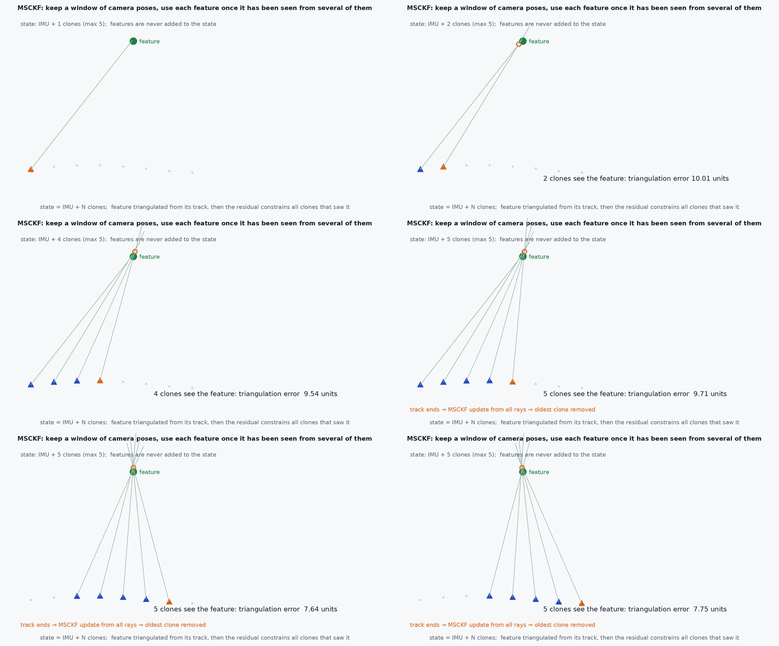
The multi-state constraint Kalman filter (MSCKF) keeps the IMU state and a sliding window of cloned past camera poses. Tracked features that are no longer seen produce constraints between the cloned poses; the feature position is never put in the filter state, but eliminated by projecting the residual into the left null space of the feature Jacobian. OpenVINS adds optional long-lived SLAM features in the state, first-estimate Jacobians for consistency, and online calibration of camera–IMU extrinsics, time offset and camera intrinsics.
Engineering intuition
A feature seen from several camera poses gives more residual equations than the 3 unknowns of its position. Three combinations of the residuals can be used to solve for the feature; the remaining combinations do not depend on the feature’s position at all: they constrain only the camera poses. Projecting onto those combinations gives clean, feature-independent constraints on the window, at a cost linear in the number of features. That is the MSCKF trick. Consistency then depends on evaluating the Jacobians at the first estimates of the states, which keeps the unobservable directions (global position and yaw) correctly unobservable (lesson M3-T12).
Mathematical formulation
For one feature with observations, the stacked linearised residual is:
The projected residual no longer depends on the feature error and gives a measurement update on the state only. The projected noise covariance is RN. has 2n − 3 columns, so a feature seen times contributes 2n − 3 independent constraints. First-estimate Jacobians: the linearisation of uses the first estimate of each state variable rather than the latest, preserving the filter’s unobservable subspace.
- Jacobian of the residual with respect to the filter state (cloned poses and calibration).
- Jacobian with respect to the feature position.
- basis of the left null space of .
Architecture and data flow
OpenVINS provides ROS 1 and ROS 2 interfaces and a configuration directory with an estimator YAML, a camera/IMU calibration YAML and an IMU noise YAML. Check the documentation pages “Getting started” and “Configuration” for the current names; the keys that matter are the camera intrinsics and extrinsics, the IMU noise densities and random walks (lesson M3-T7), the options calib_cam_extrinsics, calib_cam_timeoffset and calib_cam_intrinsics, the number of tracked features, the window size (max_clones) and the SLAM feature settings.
# estimator config excerpt (key names as in the OpenVINS documentation; verify for your version)
use_fej: true                 # first-estimate Jacobians
calib_cam_extrinsics: true    # estimate camera-IMU extrinsics online
calib_cam_timeoffset: true    # estimate camera-IMU time offset online
max_clones: 11                # size of the sliding window of camera poses
num_pts: 200                  # tracked features per frame
max_slam: 50 # long-lived SLAM features kept in the stateReal-world UAV applications
- Filter-based VIO for Capstone 1 and a comparison with optimisation-based systems.
- Online calibration of camera-IMU extrinsics and time offset.
- Embedded platforms where a filter’s predictable cost matters.
- Teaching consistency and observability.
Implementation example
This runs as shown: for a feature seen from 5 poses, the left null space of its Jacobian is computed; the projected residual has independent components and is unchanged when the feature position error changes.
import numpy as np
rng = np.random.default_rng(2)
n = 5                                                               # the feature is observed from n camera poses
Hf = rng.standard_normal((2 * n, 3))                                # feature Jacobian (2n x 3): stands for dproj/dp_f
Hx = rng.standard_normal((2 * n, 12))                               # Jacobian wrt 2 cloned poses worth of states (illustrative size)

U, s, Vt = np.linalg.svd(Hf, full_matrices=True)
N = U[:, 3:]                                                        # left null space of Hf: 2n x (2n - 3)
assert N.shape == (2 * n, 2 * n - 3) and np.allclose(N.T @ Hf, 0, atol=1e-12)

dx = rng.standard_normal(12) * 0.01; dpf_a = rng.standard_normal(3) * 0.2; dpf_b = rng.standard_normal(3) * 0.2     # two different feature position errors
r = lambda dpf: Hx @ dx + Hf @ dpf
proj_a, proj_b = N.T @ r(dpf_a), N.T @ r(dpf_b)
print("projected residual dimension:", len(proj_a), "(2n - 3 =", 2 * n - 3, ")  difference between two feature errors:", np.abs(proj_a - proj_b).max())
assert np.allclose(proj_a, proj_b, atol=1e-12) and not np.allclose(r(dpf_a), r(dpf_b))      # the feature error disappears only after projection

R = 0.5 ** 2 * np.eye(2 * n); Rp = N.T @ R @ N                                           # projected noise stays white for white input
assert np.allclose(Rp, 0.25 * np.eye(2 * n - 3), atol=1e-12)Common engineering mistakes
Disabling first-estimate Jacobians without understanding the effect
The filter gains false information about yaw and becomes overconfident.
Online calibration without excitation
Extrinsics and time offset do not converge, or converge wrongly.
Using default noise parameters from an example
Weights depend on your IMU (lesson M3-T7).
Too small a window for the motion
Features lose their baseline and the update weakens.
Assuming a filter and an optimiser behave identically
Their consistency and cost characteristics differ.
Failure modes
| Failure mode | How it shows up | Likely cause |
|---|---|---|
| Overconfident yaw | Yaw covariance shrinks with no heading source | FEJ off or a bug in the Jacobians |
| Calibration divergence | Extrinsics wander | Poor initial guess, no excitation |
| Initialisation failure | Estimate absent | Stationary start or low texture |
| High CPU | Frame drops | Too many features or SLAM features for the platform |
Debugging approach
- Run with ground truth and NEES (lesson M3-T15) to check consistency.
- Plot estimated calibration states over time.
- Check feature counts and tracking quality.
- Profile CPU against num_pts and max_slam.
Practical exercises
- Show that 2n − 3 constraints result from observations.
- Compute the null-space projection for and verify the dimension.
- Run OpenVINS on EuRoC with and without online time-offset calibration and compare.
- Read the OpenVINS documentation page on FEJ and summarise it in three sentences.
Interview questions
Write an answer in your own words, then reveal the model answer. Nothing is sent anywhere.
Question 1
What is the MSCKF trick?
Model answer
Project the feature residual into the left null space of the feature Jacobian so the update constrains only the camera poses and the feature never enters the state.
Question 2
Why first-estimate Jacobians?
Model answer
Linearising at the first estimate keeps the filter’s unobservable subspace (global position and yaw) intact, avoiding spurious information and inconsistency.
Question 3
What can OpenVINS calibrate online?
Model answer
Camera–IMU extrinsics, time offset and camera intrinsics, given enough excitation and a reasonable initial guess.
References and further reading
Primary papers, official documentation and standards. Each claim above that is specific to a tool or version points here.