UAV Systems Engineering · Module 4

M4-T4: VINS-Fusion

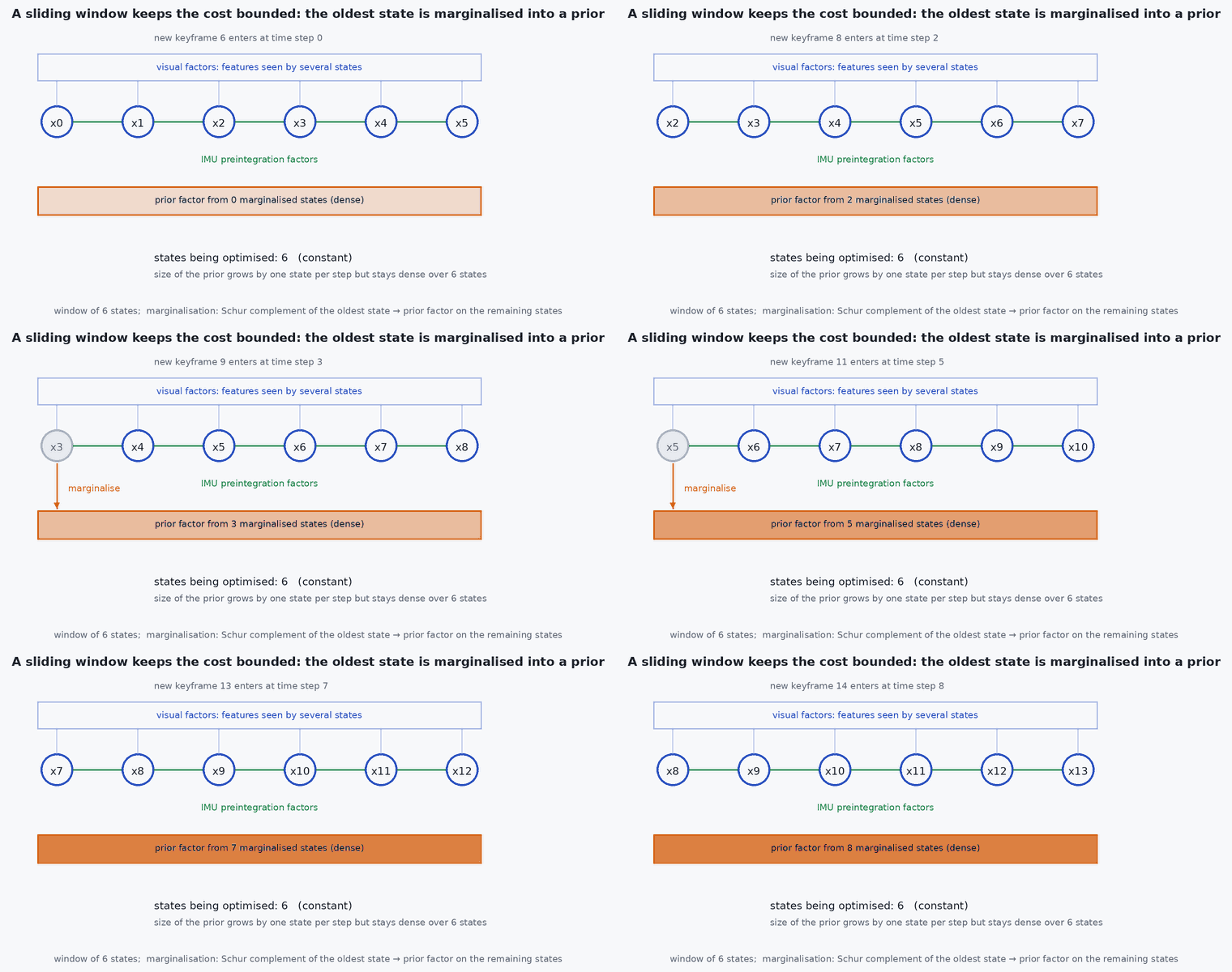
A sliding window keeps the cost bounded; marginalisation is how it forgets old states without forgetting what they taught it.

Lesson 4 of 15
SLAM and Autonomous Localization
Research-level
About 5 minutes to read

VINS-Fusion (Qin et al.) is a widely used optimisation-based estimator that supports mono and stereo cameras with an IMU, and optional GPS fusion. The idea that makes it real-time is the sliding window with marginalisation, a linear-algebra step you can verify in a few lines.

Learning objectives

After this lesson, you should be able to:

List the VINS-Fusion sensor configurations and what each estimates.
Describe the sliding-window optimisation and what is in the cost function.
Explain marginalisation via the Schur complement and verify that it preserves the information.
Run it on a dataset and state the inputs that must be configured.

Conceptual explanation

VINS-Fusion estimates states over a sliding window of recent keyframes by non-linear least squares: IMU preintegration factors between consecutive keyframes, visual reprojection factors, and a marginalisation prior summarising what older, removed states knew. Supported setups (per the repository): monocular camera + IMU, stereo, stereo + IMU, and an optional GPS fusion module that aligns the local VIO to a global frame. A separate loop-fusion node performs place recognition (DBoW2) and a 4-degree-of-freedom pose graph (the unobservable ones, lesson M3-T12).

VINS-Fusion in four blocks.

Animation of a sliding-window estimator. A chain of keyframe states is connected by inertial preintegration factors, and visual factors tie the states in the window together. As each new keyframe enters, the oldest state is marginalised: its information is folded into a prior factor on the remaining states and the state is removed, so the number of optimised states stays at six while the prior factor grows to summarise the past. — VINS-style optimisation: a window of $N$ keyframe states with IMU and visual factors; before dropping the oldest state its factors are marginalised (Schur complement) into a dense prior on the rest, which keeps the problem size fixed. Schematic of the window mechanism; counts are for a window of six. (Looping, about 6 seconds; drawn and computed for this course with illustrative values.)

Engineering intuition

Dropping an old keyframe from the window would throw away everything it constrained. Marginalisation instead integrates it out: its information about the remaining states is condensed into a prior (a quadratic term on those states). It is exact for a linear problem and a good approximation for a nonlinear one linearised once, but the linearisation point freezes at marginalisation, which is one cause of the filter inconsistency discussed in lesson M3-T12 (the first-estimate Jacobian idea is related).

Mathematical formulation

Gauss–Newton normal equations for states split into the part to keep (a) and the part to marginalise (b):

Marginalisation by the Schur complement

\begin{bmatrix}\mathbf H_{aa} & \mathbf H_{ab}\\ \mathbf H_{ba} & \mathbf H_{bb}\end{bmatrix}\begin{bmatrix}\delta\mathbf a\\ \delta\mathbf b\end{bmatrix} = \begin{bmatrix}\mathbf g_a\\ \mathbf g_b\end{bmatrix}

Marginalising b

\mathbf H^{*} = \mathbf H_{aa} - \mathbf H_{ab}\mathbf H_{bb}^{-1}\mathbf H_{ba}, \qquad \mathbf g^{*} = \mathbf g_a - \mathbf H_{ab}\mathbf H_{bb}^{-1}\mathbf g_b

The resulting (H*, g*) is the prior on the kept states. Solving the reduced system for $\delta a$ gives exactly the same $\delta a$ as solving the full system, which is the property the test below verifies. Visual factors use reprojection residuals (lesson M4-T2); IMU factors use the preintegrated residuals and bias random walk (lesson M3-T8); keyframe and marginalisation policy depends on parallax and tracking quality.

$H$ , $g$: Hessian approximation $J^{\top}$ WJ and gradient of the least-squares problem.
H*: information (prior) on the kept states after marginalisation.

Architecture and data flow

Typical launch (from the repository README; check the version): the estimator node reads a YAML configuration with camera and IMU topics, calibration (intrinsics, extrinsic rotation and translation camera–IMU, time offset estimation flags) and IMU noise parameters.

# ROS 1 workspace with VINS-Fusion built
roslaunch vins vins_rviz.launch
rosrun vins vins_node ~/catkin_ws/src/VINS-Fusion/config/euroc/euroc_stereo_imu_config.yaml
rosrun loop_fusion loop_fusion_node ~/catkin_ws/src/VINS-Fusion/config/euroc/euroc_stereo_imu_config.yaml
rosbag play MH_01_easy.bag

Run sequence from the README (ROS 1). Check ROS 2 ports separately if needed.

# excerpt of a VINS-Fusion configuration (key names as in the shipped EuRoC configs)
imu_topic: "/imu0"
image0_topic: "/cam0/image_raw"
image1_topic: "/cam1/image_raw"
estimate_extrinsic: 1      # 0: trust the extrinsics, 1: refine around an initial guess, 2: calibrate from scratch
estimate_td: 1             # estimate the camera-IMU time offset online
acc_n: 0.08                # accelerometer noise density (use YOUR sensor)
gyr_n: 0.004

Calibration and noise parameters decide the quality; do not copy example values blindly.

Real-world UAV applications

Stereo-inertial odometry for Capstone 1.
Global trajectory alignment with GPS when available.
Research baseline against OpenVINS and ORB-SLAM3.
Studying marginalisation and sliding-window design.

Implementation example

This runs as shown: a small linear least-squares problem (a chain of 1-D states) is solved in full and again after marginalising the first two states by the Schur complement; the kept states agree exactly.

import numpy as np
rng = np.random.default_rng(3)
n = 6                                                               # states x0..x5 (a 1-D trajectory), measured by odometry between neighbours and by two absolute fixes
rows, y = [], []
for i in range(n - 1):
    r = np.zeros(n); r[i], r[i + 1] = -1, 1; rows.append(r); y.append(1.0 + 0.05 * rng.standard_normal())     # x_{i+1} - x_i = 1
for i, v in ((0, 0.0), (5, 5.0)):                                  # absolute fixes at the ends
    r = np.zeros(n); r[i] = 1; rows.append(r * 3.0); y.append(3.0 * v + 0.05 * rng.standard_normal())
J = np.array(rows); y = np.array(y); H = J.T @ J; g = J.T @ y
x_full = np.linalg.solve(H, g)

keep, marg = [2, 3, 4, 5], [0, 1]                                  # marginalise the oldest two states
Haa, Hab, Hbb = H[np.ix_(keep, keep)], H[np.ix_(keep, marg)], H[np.ix_(marg, marg)]
Hstar = Haa - Hab @ np.linalg.solve(Hbb, Hab.T)
gstar = g[keep] - Hab @ np.linalg.solve(Hbb, g[marg])
x_keep = np.linalg.solve(Hstar, gstar)
print("full:", np.round(x_full[keep], 6), "\nmarginalised:", np.round(x_keep, 6))
assert np.allclose(x_full[keep], x_keep, atol=1e-10)
assert np.all(np.linalg.eigvalsh(Hstar) > 0)                        # the prior is a valid (positive definite) information matrix

Marginalisation by the Schur complement preserves the solution for the kept states.

Common engineering mistakes

Copying the example IMU noise values

They belong to another sensor; weights depend on them (lesson M3-T7).

Leaving extrinsics and time offset at defaults

Wrong values cause drift in fast motion (lessons M7-T8, M7-T16).

Not enough excitation to initialise

Move gently at start to observe scale and gravity.

Using the loop-closed pose for control

It jumps: use the local VIO output.

Assuming ROS 1 Noetic-style launch works on ROS 2

Use a maintained ROS 2 port and check its interface.

Failure modes

Failure modes, symptoms and causes
Failure mode	How it shows up	Likely cause
Drift in fast manoeuvres	Estimate wanders when turning	Time offset or extrinsic error
Initialisation failure	No estimate at start	Stationary start, no excitation
Window too small	Early drift and inconsistency	Insufficient window for the motion
Frame mismatch with PX4	Mirrored trajectory in flight	ENU/FLU versus NED/FRD conversion (lesson M6-T10)

Debugging approach

Check feature count and tracking in the visualiser.
Plot estimated time offset and biases.
Evaluate with evo against ground truth.
Verify topic names, rates and timestamps.

Practical exercises

Run the EuRoC stereo-inertial configuration and compute ATE.
Set estimate_td to 0 and add an artificial 20 ms delay to the images: compare.
Verify marginalisation on a nonlinear problem and see where linearisation matters.
List the configuration values that must come from your own calibration.

Interview questions

Write an answer in your own words, then reveal the model answer. Nothing is sent anywhere.

Question 1

Why a sliding window?

Model answer

It bounds the optimisation cost to recent keyframes; older states are marginalised into a prior that keeps their information.

Question 2

What is marginalisation?

Model answer

Eliminating states from the problem by the Schur complement, summarising their effect on the remaining states as a prior, exact in the linear case.

Question 3

What does VINS-Fusion’s loop closure estimate?

Model answer

A four-degree-of-freedom pose graph (three translations and yaw), because roll, pitch and scale are observable and already well constrained.

References and further reading

Primary papers, official documentation and standards. Each claim above that is specific to a tool or version points here.

What’s next

Mark this lesson

Saved in this browser and synced to your account when you are signed in.

Next lesson

M4-T5: OpenVINS

Describe the MSCKF-based OpenVINS estimator, its state, and how it differs from sliding-window optimisation.