UAV Systems Engineering · Module 4
M4-T1: SLAM fundamentals
To map you need to know where you are, and to know where you are you need a map: SLAM solves both together, and the correlations are the whole story.
Simultaneous localisation and mapping is the framework behind ORB-SLAM3, VINS-Fusion, LIO-SAM and FAST-LIVO2. Its essential insight is statistical: the robot’s error and the map’s errors are correlated, and revisiting a place propagates information through those correlations to the whole trajectory.
Learning objectives
After this lesson, you should be able to:
- State the SLAM problem and the roles of front-end and back-end.
- Explain why the robot and landmark errors are correlated and what a loop closure does.
- Run a one-dimensional EKF-SLAM example and observe the correlations.
- Distinguish filtering and smoothing formulations, and odometry from SLAM.
Conceptual explanation
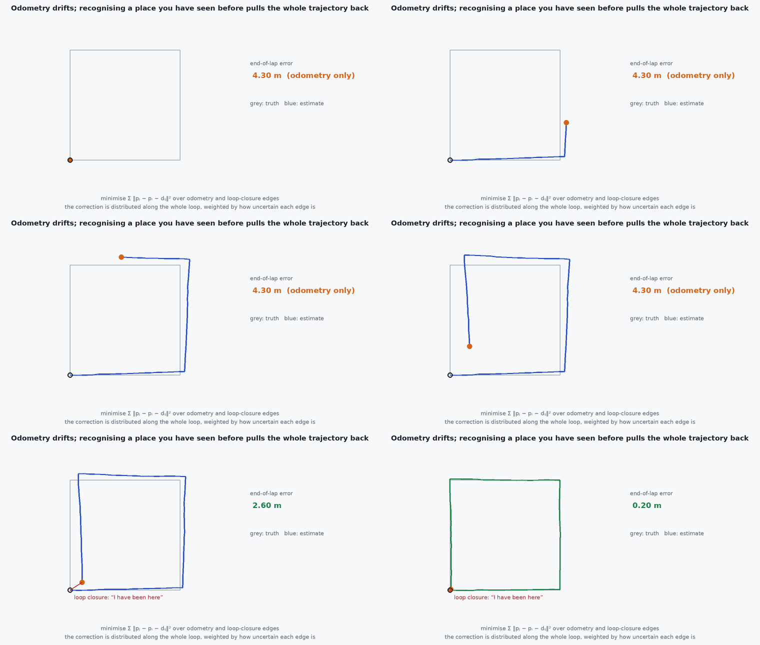
SLAM estimates the vehicle trajectory and a map from controls and observations . The front-end turns raw sensor data into constraints: feature tracks, scan matches, data associations and loop-closure candidates. The back-end estimates the trajectory and map from those constraints, by filtering (EKF, particle) or by smoothing (pose graph, bundle adjustment, factor graph). Odometry is SLAM without loop closure: it accumulates drift; loop closure recognises a revisited place and removes it.
Engineering intuition
Every landmark position is measured relative to where the robot was, so an error in the robot’s pose becomes the same error in the landmarks seen from it: they are correlated. When the robot later sees an old landmark again, the measurement tightens that landmark and, through the correlation, also tightens the robot’s own position and every landmark seen alongside it. That is why one loop closure can correct a long trajectory: information flows along the correlations. It is also why a false loop closure is so destructive: it injects confident wrong information into all those links.
Mathematical formulation
Full SLAM posterior and its factorisation (Markov assumptions):
Taking the negative log with Gaussian noise gives the nonlinear least-squares problem solved by the back-end (pose graphs: lesson M4-T12; bundle adjustment: lesson M4-T2):
EKF-SLAM keeps the joint Gaussian over the current pose and all landmarks, with a covariance that has off-diagonal robot–landmark and landmark–landmark blocks; its cost grows quadratically with the number of landmarks, which is why modern systems use sparse smoothing instead. Marginalising old states creates dense blocks (fill-in), the reason for keyframes and sliding windows.
- robot pose at time .
- map (landmarks, voxels or point cloud).
- ,
- motion and observation models.
- ,
- motion and measurement noise covariances.
Architecture and data flow
On a UAV: VIO or LIO gives smooth, high-rate local odometry; a SLAM layer adds loop closure and maintains a globally consistent map, publishing a correction as the transform between the map frame and the odom frame (as in the ROS convention). The controller consumes the odom-frame estimate (smooth, no jumps); the planner and mission layer use the map-frame estimate. Never feed a jumping map-frame pose directly to the controller.
Real-world UAV applications
- Building maps of unknown environments for later localisation (lesson M4-T13).
- Drift correction on long GNSS-denied flights.
- Multi-session mapping and map merging.
- Obstacle maps for planning.
Implementation example
This runs as shown: a one-dimensional EKF-SLAM with a robot and two landmarks. The robot drives away and back; re-observing the first landmark shrinks the robot’s variance and the correlation between robot and landmark is non-zero throughout.
import numpy as np
rng = np.random.default_rng(0)
true_L = np.array([5.0, 12.0]); q, r = 0.2, 0.15                    # motion noise per step, measurement noise
x = np.array([0.0, 4.0, 11.0]); P = np.diag([0.0, 4.0, 4.0])       # state: robot, landmark 1, landmark 2 (landmarks start badly known)
truth = 0.0; trace = []

def update(x, P, j, z):                                           # measurement z = L_j - robot
    H = np.zeros((1, 3)); H[0, 1 + j] = 1; H[0, 0] = -1
    S = H @ P @ H.T + r ** 2; K = P @ H.T / S
    x = x + (K * (z - (x[1 + j] - x[0]))).ravel(); P = (np.eye(3) - K @ H) @ P @ (np.eye(3) - K @ H).T + K @ np.array([[r ** 2]]) @ K.T
    return x, P

for k in range(120):
    u = 0.15 if k < 60 else -0.15                                   # drive out for 60 steps, then back for 60
    truth += u + q * rng.standard_normal()
    x[0] += u; P[0, 0] += q ** 2                                   # prediction: only the robot moves, landmarks are static
    for j in (0, 1):
        if abs(true_L[j] - truth) < 6.0: x, P = update(x, P, j, true_L[j] - truth + r * rng.standard_normal())
    trace.append((P[0, 0], P[0, 1], P[1, 1]))
rho = P[0, 1] / np.sqrt(P[0, 0] * P[1, 1])
print(f"final robot std {np.sqrt(P[0, 0]):.3f} m, landmark-1 std {np.sqrt(P[1, 1]):.3f} m, robot-landmark correlation {rho:.2f}")
print(f"robot position error {abs(x[0] - truth):.3f} m, landmark errors {np.round(np.abs(x[1:] - true_L), 3)}")
assert abs(rho) > 0.3                                               # robot and landmark errors are correlated
assert np.sqrt(P[1, 1]) < 0.5 * 2.0 and abs(x[0] - truth) < 0.5     # the map and robot both became well known (landmarks started with std 2 m)
assert np.sqrt(trace[-1][0]) < np.sqrt(max(t[0] for t in trace)) # robot uncertainty shrank after revisiting landmark 1Common engineering mistakes
Treating SLAM as odometry with a map attached
The loop-closure and consistency machinery is what distinguishes it.
Accepting any loop closure
A false positive can ruin the map: verify geometrically.
Feeding map-frame jumps to the controller
Use the continuous odom-frame estimate for control.
Unbounded map growth
Keyframes, culling and voxel filtering are required for a bounded compute budget.
Ignoring dynamics
Moving objects corrupt the map; filter or model them.
Failure modes
| Failure mode | How it shows up | Likely cause |
|---|---|---|
| Map distortion after a false loop | Folded or doubled structures | Perceptual aliasing, weak verification |
| Tracking loss | System reinitialises or runs on IMU alone | Fast motion, low texture, dynamic scene |
| Inconsistent map | Doubled walls | No loop closure or timing errors |
| Compute explosion | Latency grows over a long flight | Map not bounded |
Debugging approach
- Plot the trajectory before and after loop closure and the covariance trend.
- Review every accepted loop with geometric verification statistics.
- Check the map for double surfaces.
- Log tracking state and compute time.
Practical exercises
- Show analytically why re-observing landmark 1 reduces the robot variance in the 1-D example.
- Add a false loop (a wrong association) to the example and observe the damage.
- Estimate the EKF-SLAM cost for 1000 landmarks and compare with a sparse smoother.
- Describe the map-to-odom transform and who publishes it.
Interview questions
Write an answer in your own words, then reveal the model answer. Nothing is sent anywhere.
Question 1
What are the front-end and back-end of a SLAM system?
Model answer
The front-end extracts constraints from sensor data (tracking, matching, loop candidates); the back-end estimates the trajectory and map from those constraints by filtering or optimisation.
Question 2
Why are robot and landmark errors correlated?
Model answer
Landmarks are measured relative to the robot pose, so any error in the pose appears in all landmarks seen from it; revisiting a landmark therefore corrects the pose and the other landmarks through the correlations.
Question 3
What is the difference between VO/VIO and SLAM?
Model answer
Odometry accumulates drift; SLAM adds recognition of revisited places and global optimisation to remove it.
References and further reading
Primary papers, official documentation and standards. Each claim above that is specific to a tool or version points here.
- C. Cadena et al., “Past, present, and future of simultaneous localization and mapping: toward the robust-perception age”, IEEE T-RO, 2016
- . Thrun, . Burgard, . Fox, Probabilistic Robotics, MIT Press, 2005, chapters 10–13.
- G. Grisetti et al., “A tutorial on graph-based SLAM”, IEEE ITS Magazine, 2010