UAV Systems Engineering · Module 4
M4-T2: Visual SLAM
Visual SLAM keeps a sparse set of keyframes and 3-D points and keeps refining both so that every point projects where it was seen.
The back-bone of feature-based visual SLAM is bundle adjustment: adjust camera poses and 3-D points together to minimise reprojection error. Understanding what it optimises, what it holds fixed and why it is run on a window explains most of the design of ORB-SLAM3 and VINS-Fusion.
Learning objectives
After this lesson, you should be able to:
- Describe keyframes, map points and the covisibility graph.
- Write the reprojection error and the bundle adjustment objective.
- Explain the gauge freedoms and why local (windowed) and global BA are used.
- Run a small bundle adjustment and verify that it reaches the noise level.
Conceptual explanation
A feature-based visual SLAM system tracks features in every frame, but stores only keyframes (frames that add new information, chosen by parallax or tracked-feature ratio) and map points (triangulated 3-D landmarks with descriptors). The covisibility graph links keyframes that see common points; local optimisation works on a keyframe and its neighbours. Bundle adjustment (BA) refines poses and points jointly to minimise reprojection error.
Engineering intuition
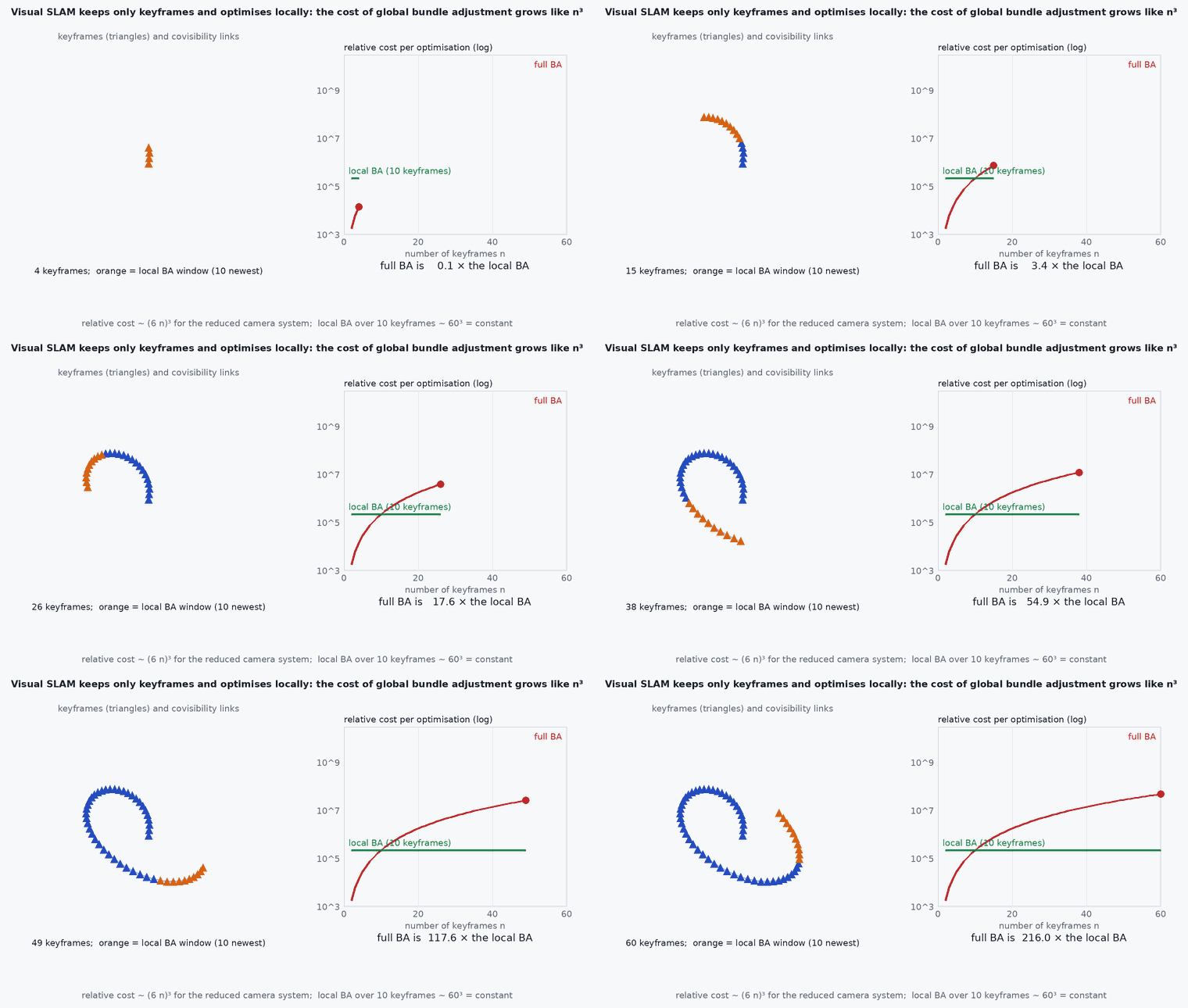
Each observation of a point in a keyframe is a ray; the point sits where the rays from different keyframes intersect. With noisy poses the rays do not meet; BA moves the poses and the points until the rays are as consistent as the measurement noise allows. The more keyframes see the point from different viewpoints, the better it is constrained; points seen only from one viewpoint (pure rotation) carry no depth information. Because BA is expensive (cost grows rapidly with the number of keyframes), the local version optimises only recent keyframes and the points they see, while older ones are held fixed or marginalised.
Mathematical formulation
The reprojection error of point in keyframe with pose , intrinsics and observed pixel , and the BA objective:
is a robust kernel (Huber) limiting the influence of outliers. The Jacobian is sparse: each residual involves one pose and one point. The normal equations have the arrow structure that is solved efficiently by the Schur complement (eliminate the points first, solve for the poses, back-substitute). Gauge freedom: a global rigid transform leaves every reprojection error unchanged (six degrees of freedom), and for a monocular system, a global scale also (seven): fix the first pose and one distance, or use priors, as the example does. Cost per iteration is dominated by the reduced camera system, in the number of poses, hence the windows.
- projection of the 3-D point into the camera: transform by , divide by depth, apply .
- pixel noise covariance.
- robust loss.
Architecture and data flow
Frontend: feature extraction and matching (ORB, in ORB-SLAM3; Shi–Tomasi with optical flow in VINS-Fusion), pose tracking by motion-only BA, keyframe decision. Back-end: local BA on the covisibility neighbourhood, global BA or pose-graph optimisation on loop closure. Output: keyframe poses and a sparse point map; dense maps need a separate module. The IMU enters as preintegration factors in the visual-inertial versions (lesson M3-T8).
Real-world UAV applications
- Feature-based SLAM with ORB-SLAM3 and VINS-Fusion.
- Photogrammetric reconstruction (structure from motion).
- Calibrating a camera rig by BA on a calibration target.
- Offline refinement of a flown trajectory.
Implementation example
This runs as shown: a planar bearing-only bundle adjustment with 6 poses and 25 landmarks. The chi-square (twice the cost) falls to about the number of degrees of freedom, i.e. the noise level, and landmark error halves. The numerical Jacobian keeps the example short; real systems use analytic sparse Jacobians and the Schur complement.
import numpy as np
rng = np.random.default_rng(1)
wrap = lambda a: (a + np.pi) % (2 * np.pi) - np.pi
K, M = 6, 25
poses = np.array([[1.5 * k, 0.3 * np.sin(k), 0.05 * k] for k in range(K)])          # true camera poses (x, y, heading)
pts = np.stack([rng.uniform(0, 9, M), rng.uniform(3, 8, M)], axis=1)               # true landmarks
bearing = lambda p, l: wrap(np.arctan2(l[1] - p[1], l[0] - p[0]) - p[2])
sig = np.radians(0.5)
obs = [(k, j, bearing(poses[k], pts[j]) + sig * rng.standard_normal()) for k in range(K) for j in range(M)]

init_p = poses + np.array([0.15, 0.15, 0.03]) * rng.standard_normal((K, 3)) * np.arange(K)[:, None] / 2
init_p[0] = poses[0]; init_p[1, :2] = poses[1, :2]                                  # gauge: pose 0 and the position of pose 1 fixed (fixes scale)
init_l = pts + 0.6 * rng.standard_normal((M, 2))
unpack = lambda x: (x[:3 * K].reshape(K, 3), x[3 * K:].reshape(M, 2))

def resid(x):
    P, L = unpack(x)
    r = [wrap(bearing(P[k], L[j]) - z) / sig for k, j, z in obs]
    r += list((P[0] - poses[0]) * 1e4) + list((P[1, :2] - poses[1, :2]) * 1e4)      # gauge priors
    return np.array(r)

x = np.concatenate([init_p.ravel(), init_l.ravel()])
cost0 = 0.5 * np.sum(resid(x) ** 2); lm_err0 = np.mean(np.linalg.norm(unpack(x)[1] - pts, axis=1))
for it in range(20):                                                                # Gauss-Newton with numerical Jacobians
    r = resid(x); J = np.zeros((len(r), len(x)))
    for i in range(len(x)):
        xp = x.copy(); xp[i] += 1e-6; J[:, i] = (resid(xp) - r) / 1e-6
    dx = np.linalg.solve(J.T @ J + 1e-6 * np.eye(len(x)), -J.T @ r); x += dx
    if np.linalg.norm(dx) < 1e-9: break
cost = 0.5 * np.sum(resid(x) ** 2); lm_err = np.mean(np.linalg.norm(unpack(x)[1] - pts, axis=1))
dof = len(obs) - (3 * K - 3 + 2 * M - 2)                                            # residuals minus free parameters
print(f"cost {cost0:.0f} -> {cost:.1f}, chi-square {2 * cost:.0f} (degrees of freedom {dof}); landmark error {lm_err0:.2f} -> {lm_err:.2f} m")
assert cost < cost0 / 50 and 0.6 * dof < 2 * cost < 1.5 * dof and lm_err < 0.7 * lm_err0Common engineering mistakes
Running global BA online
Cost grows quickly with keyframes; use local windows and pose-graph for loops.
No outlier handling
A few wrong matches distort the solution: robust kernels and RANSAC.
Free gauge
Singular normal equations: fix a pose and the scale.
Too many keyframes
Compute explodes; cull redundant keyframes and points.
Pure rotation initialisation
No parallax: depth unobservable, bad initial map.
Failure modes
| Failure mode | How it shows up | Likely cause |
|---|---|---|
| Tracking lost | No pose | Blur, low texture, fast motion |
| Scale drift (monocular) | Map size changes | No scale constraint; add stereo or IMU |
| Bad initialisation | Map collapsed or flat | Insufficient parallax |
| Map corruption | Moving objects mapped as static | No dynamic filtering |
Debugging approach
- Plot reprojection error per observation to find outliers.
- Check the number of map points per keyframe.
- Examine keyframe rate and parallax.
- Compare against a dataset with ground truth.
Practical exercises
- Derive the Jacobian of the bearing residual with respect to the pose and point.
- Add a few gross outlier bearings to the example and compare plain and Huber-weighted BA.
- Count the gauge freedoms of a monocular BA.
- Estimate the cost of the reduced camera system for 100 keyframes.
Interview questions
Write an answer in your own words, then reveal the model answer. Nothing is sent anywhere.
Question 1
What does bundle adjustment minimise?
Model answer
The sum of squared (robustified) reprojection errors over all observations, by adjusting camera poses and 3-D points jointly.
Question 2
Why are local windows used?
Model answer
BA cost grows rapidly with the number of keyframes, so only recent keyframes and the points they see are optimised online, with the rest fixed or marginalised.
Question 3
What gauge freedoms does monocular BA have?
Model answer
Global rotation and translation (six) and scale (one): fixed by anchoring a pose and a distance or by priors.
References and further reading
Primary papers, official documentation and standards. Each claim above that is specific to a tool or version points here.
- B. Triggs, P. McLauchlan, R. Hartley, A. Fitzgibbon, “Bundle adjustment: a modern synthesis”, Vision Algorithms 1999
- R. Mur-Artal, J. M. M. Montiel, J. D. Tardós, “ORB-SLAM: a versatile and accurate monocular SLAM system”, IEEE T-RO, 2015
- Ceres Solver documentation: nonlinear least squares and bundle adjustment